Your building management system is logging temperature, flow, and energy data around the clock. But if no one knows how to translate those numbers into control decisions, the meters are just expensive record-keepers.
This guide gives facilities managers, HVAC technicians, and building engineers a practical, step-by-step workflow for interpreting thermal mass meter readings — from raw data to actionable setpoint adjustments. Whether you manage a single commercial office or a multi-site campus, the same interpretation framework applies: establish a baseline, identify patterns, correlate readings to HVAC events, and act on what you find.
By the end of this guide you will be able to recognize the three most common meter-reading patterns (lag, ramp, and hysteresis), understand what they tell you about your building’s thermal behaviour, and apply that knowledge to reduce energy waste, cut peak demand charges, and improve occupant comfort — without adding new sensors or replacing existing equipment.
Understanding Thermal Mass Basics
What Thermal Mass Is and How It Affects Building Thermal Behaviour
Thermal mass refers to a building material’s ability to absorb heat energy, store it, and release it slowly over time. Concrete floors, brick walls, water-filled pipes, and structural steel all act as thermal batteries — charging during periods of high heat input and discharging when the surrounding temperature drops. The governing property is heat capacity (specific heat × density × volume), measured in kJ/K or BTU/°F per unit volume.
For HVAC engineers, the practical consequence is this: the temperature inside a high-mass building does not track outdoor temperature in real time. A 200 mm concrete slab in a south-facing office wall can absorb solar heat all morning and not release it into the occupied space until mid-afternoon. By then, the HVAC system is fighting both the residual heat load from the slab and the peak occupancy load — a double penalty that flat, occupancy-based schedules never anticipate.
A 2025 study published in Energy for Sustainable Development (ScienceDirect) found that thermal mass in commercial buildings tends to store heat when it is not needed and release it when buildings do not require it — the opposite of optimal behaviour. The remedy is not more insulation; it is smarter control informed by accurate meter data that reveals when mass is charging and discharging.
Different Materials and Their Storage Capacities
Not all thermal mass behaves the same way. The table below summarises the volumetric heat capacity and typical thermal lag (the time delay between peak outdoor temperature and peak indoor surface temperature) for materials commonly found in commercial buildings.
| Material | Density (kg/m³) | Specific Heat (kJ/kg·K) | Volumetric Heat Capacity (kJ/m³·K) | Typical Thermal Lag (hours) | Common Location in Buildings |
|---|---|---|---|---|---|
| Reinforced concrete | 2,400 | 0.88 | 2,112 | 8–12 | Structural slabs, walls, columns |
| Dense brick | 1,800 | 0.84 | 1,512 | 6–10 | External walls, partition walls |
| Water (in chilled water system) | 1,000 | 4.18 | 4,180 | 1–3 (fast responding) | Chilled-water loops, thermal storage tanks |
| Timber (softwood) | 500 | 1.60 | 800 | 2–4 | Floors, cladding, furniture |
| Steel (structural) | 7,800 | 0.50 | 3,900 | 1–2 (fast releasing) | Exposed structural frames, metal decking |
| Gypsum plasterboard | 900 | 0.84 | 756 | 1–2 | Internal wall linings |
| Phase-change material (PCM) board | 800–1,000 | ~100–200 (latent, at transition) | 80,000–200,000 (latent) | 2–5 (engineered) | Retrofit insulation boards, ceiling tiles |
Table 1: Volumetric heat capacity and thermal lag for common building materials. PCM values reflect effective latent heat storage at phase-transition temperature. Sources: Wikipedia – Thermal Mass; MIT OpenCourseWare 4.401; ScienceDirect energy studies.
How Accumulation and Release of Heat Relate to HVAC Demand
The link between thermal mass and HVAC demand works like a capacitor in an electrical circuit: it smooths peaks but also delays them. During the charging phase (heat flowing into mass), the HVAC cooling load appears lower than the actual heat input — the structure absorbs the surplus. During the discharging phase (heat flowing out of mass back into the space), the cooling load spikes above what the instantaneous heat sources alone would predict.
This is why a building that maintained 22°C all day through an August heatwave may suddenly require 30% more cooling tonnage at 6 PM — long after solar gain has subsided. The thermal mass is discharging stored heat into the occupied zone. Without a meter that captures this delayed load, control systems running on real-time occupancy sensors alone will always be reacting too slowly. Understanding this mechanism is the first step to using meter data proactively rather than reactively.
What Meter Readings Measure
 Modern BMS dashboards aggregate temperature, flow, and derived heat-transfer readings from multiple sensors — but interpretation requires knowing what each variable actually represents.
Temperature, Capacitance, and Flow Data
A thermal mass meter typically reports three primary variables: supply temperature (Ts), return temperature (Tr), and volumetric or mass flow rate (Q). From these three values, the meter computes thermal power (P) using the fundamental heat transfer equation:
P = Q × ρ × cp × (Ts − Tr) [watts or BTU/hr]
Where ρ is fluid density and cp is specific heat capacity. This equation means that a reading error in any one of the three variables compounds into the final energy figure — a 1% error in flow rate combined with a 0.5°C temperature drift can produce a 5–8% error in the reported thermal power, which at the scale of a 500 kW chilled-water plant represents 25–40 kW of undetected waste.
In some installations, the meter also reports thermal capacitance — an indicator of how much heat energy the monitored circuit is currently absorbing per degree of temperature change. A rising capacitance reading during a steady flow period indicates that mass is charging. A falling capacitance at the same flow rate means mass is discharging. This derived variable is the closest thing to a direct window into the building’s thermal battery state.
Time Scales: Short-Term vs Long-Term Readings
The same meter reading can mean very different things depending on the time window you examine it through. A 5-minute snapshot captures instantaneous demand — useful for diagnosing a stuck valve or confirming a setpoint change has taken effect. A 24-hour trend reveals daily charging and discharging cycles — essential for setback scheduling. A 30-day rolling average separates systematic patterns from weather-driven anomalies — the baseline for performance benchmarking.
Most BMS platforms store meter data at 5- to 15-minute intervals, which is adequate for trend analysis. For equipment fault detection — identifying a heat exchanger fouling or a pump operating at wrong duty — 1-minute resolution is preferred. Facilities teams that rely only on hourly data lose the transient signals (rapid flow drops, sharp temperature spikes) that indicate developing faults before they become costly failures.
Data Quality Considerations: Noise, Calibration, and Placement
Before interpreting any reading, verify three data quality preconditions:
- Calibration status: Temperature sensors (RTDs) drift by 0.1–0.3°C per year. On a ΔT of 5°C (typical for chilled-water metering), a 0.5°C sensor pair drift is a 10% energy-reading error. The Sage Metering calibration guide recommends annual in-situ verification for all critical energy metering points.
- Signal noise: Flow meter signals with high-frequency noise (fluctuations faster than 10 seconds) indicate hydraulic turbulence near the sensor — typically caused by proximity to a valve, pump discharge, or elbow. These need signal filtering or sensor relocation, not control response.
- Sensor placement: Temperature sensors must be installed downstream of thorough mixing — at least 5D (pipe diameters) beyond any tee, reducing fitting, or heat exchanger outlet. A sensor placed 1D from a mixing valve will read the temperature of whichever inlet stream dominates at that moment, not the mixed supply temperature. The result is wild apparent ΔT swings that look like demand spikes but are pure measurement artefacts.
Preparing for Interpretation
Setting Baseline Expectations for Your Building
A baseline is the meter profile your building produces under known, stable conditions — full occupancy, standard weather, no abnormal equipment events. Without a baseline, every reading is ambiguous: is today’s 15% higher energy use a real load increase, or is it because yesterday was unusually cool? The baseline answers that question by providing context.
To establish a useful baseline, collect 20–30 days of consecutive meter data during a representative period — typically mid-season (March–April or September–October in temperate climates) when neither heating nor cooling dominates. Exclude days with anomalous occupancy (holidays, shutdowns), unusual weather (extreme heat or cold events), or known equipment issues. The resulting daily load profile, plotted as thermal power versus time of day, becomes your reference template.
Defining Periods of Interest: Peak Loads, Shoulder Seasons, Setbacks
Three periods in the daily and annual meter record deserve systematic analysis:
- Peak load periods: The hours of highest thermal demand (typically 10:00–15:00 for cooling, 07:00–09:00 for heating). Meter behaviour during peak periods reveals whether thermal mass is amplifying or buffering demand — a critical distinction for sizing backup capacity and managing utility demand charges.
- Shoulder seasons (spring, autumn): Free-cooling potential is highest. Meter readings that show cooling demand persisting into mild-weather periods despite low outdoor temperatures indicate thermal mass discharging stored summer heat — a common finding in heavyweight construction with poor overnight ventilation strategies.
- Setback periods: The night-time or unoccupied hours when HVAC is reduced or off. How quickly the building cools down (and heats back up on restart) is a direct measurement of the building’s thermal mass. A building that cools by only 2°C overnight despite 10°C external temperatures has very high thermal mass — and therefore a large pre-cooling opportunity (discussed in Section 7).
Data Cleansing and Synchronisation Across Sensors
Raw BMS data is rarely clean. Common issues include: sensor timeouts producing NULL values (which average-to-zero and distort totals), clock synchronisation offsets between sensors (a 5-minute offset between the supply temperature and flow rate sensors produces artificial energy spikes), and unit mismatches (a flow sensor returning L/min while the meter expects m³/h will compute 1000× the correct energy value). Before any analysis, run a data quality check: plot each raw signal independently, confirm units match the meter’s configuration, and verify timestamps align within 30 seconds across all sensor channels.
Step-by-Step Interpretation Workflow
 The interpretation workflow moves from data collection and baseline establishment through pattern recognition to control action — each step building on the one before it.
Gather data and establish a baseline. Export 30 days of meter data at 5-minute resolution: supply temperature, return temperature, flow rate, and derived thermal power. Plot the average weekday load profile (thermal power vs. time of day). This profile is your baseline. Flag any days that deviate by more than ±15% at the same time of day — these are candidates for deeper investigation, not drivers of the baseline itself.
Map readings to HVAC events. Overlay the meter data with your BMS event log: AHU start/stop times, setpoint changes, valve actuations, economiser enable/disable events, and reset cycles. Each HVAC event should produce a visible signature in the meter data — a flow step change on pump start, a ΔT step on setpoint adjustment, or a gradual slope on economiser engagement. If an event produces no signature, either the meter is not in the right location to measure it, or the actuator did not respond as commanded. Both are valuable findings.
Identify lag, ramp, and hysteresis patterns. With the event map in place, examine the meter trace for three specific shapes: (a) Lag — a time delay between a control signal change and a corresponding meter response, measured in minutes; (b) Ramp — a gradual, linear increase or decrease in thermal power over 1–4 hours, indicating mass charging or discharging; (c) Hysteresis — a difference in the meter trace between heating-up and cooling-down cycles at the same set conditions, indicating that the thermal mass is responding differently depending on the direction of temperature change. All three patterns have specific implications for control strategy, discussed in Section 5.
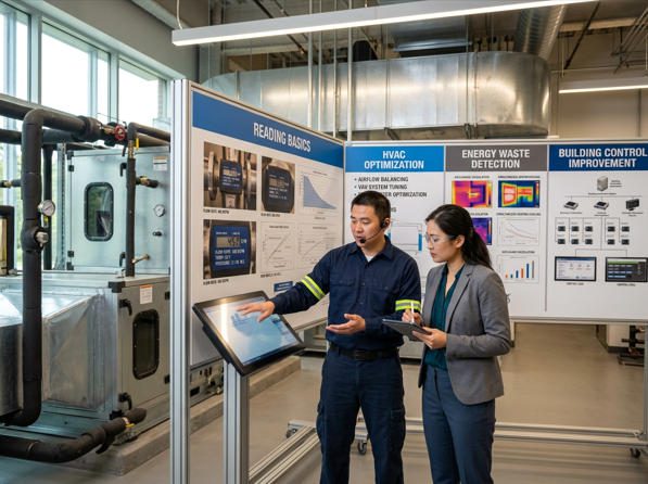
▶ How thermal mass flow meter technology works — including signal interpretation and measurement principles relevant to HVAC applications. Credit: Sierra Instruments.
Identifying Common Reading Patterns
High Lag with Slow Recovery: What It Means for Cooling or Heating Control
Thermal lag in a meter trace looks like this: the outdoor temperature peaks at 14:00, but the building’s cooling demand (as measured by the chilled-water meter) does not peak until 18:00 or later. The four-hour offset is the lag — the time taken for heat to conduct through the thermal mass and appear as a sensible load on the HVAC system.
High lag with slow recovery is the signature of a high-mass building (dense concrete, full-height masonry) that has absorbed a large heat load. When you see this pattern, the control implication is clear: your AHU setpoints and cooling schedules need to anticipate the delayed peak, not react to it. Running cooling at full capacity from 07:00 to 17:00 and cutting back at building closure time will leave occupants uncomfortable in the final hour while the meter — correctly — shows rising demand. The fix is to extend cooling capacity 2–3 hours before the anticipated discharge peak, informed by the lag time measured from your baseline data.
Low Thermal Mass Conditions and Their Implications for Control Strategies
At the opposite end, lightweight buildings (steel frame with glass curtain wall, suspended ceiling, carpet tiles) show very low thermal lag — typically under 1 hour. Their meter traces track outdoor conditions almost in real time. The advantage is fast response to control changes: lower a setpoint by 1°C and the meter confirms reduced demand within 20 minutes. The disadvantage is vulnerability to rapid load swings: a cloud passing over a south-facing façade can drop the cooling load by 15% in 5 minutes, causing a VAV system to over-deliver cold air and create discomfort before the controls react. For low-mass buildings, the control priority is tight proportional-integral (PI) gains and fast meter polling intervals (1-minute resolution or better) to keep pace with the building’s rapid thermal response.
Anomalies Indicating Sensor or System Faults
Three anomalous meter patterns reliably indicate a hardware fault rather than a real process change:
- Step jump with no corresponding HVAC event: Flow rate increases by 20% in one 5-minute polling interval without any pump speed change or valve actuation in the event log. Probable cause: a stuck check valve has opened, or a secondary pump has started in an unmonitored circuit. Investigate hydraulically.
- ΔT collapse to near zero at steady flow: Supply and return temperatures converge rapidly (ΔT drops from 6°C to 0.5°C) with no change in flow. Probable cause: a bypass valve has opened and is short-circuiting the chilled-water distribution loop, bypassing the coils. This is a serious fault — the meter reading will show near-zero thermal output while the chiller is running at full capacity, wasting the energy cost of generating chilled water that never reaches the load.
- Periodic flat-line periods: The meter shows exactly the same value (to three decimal places) for 15–30 minute stretches at irregular intervals. This is almost always a sensor communication timeout producing the last-held value — a data quality artefact, not a real flat-load condition. Check sensor wiring, battery backup, and BMS polling configuration.
Correlating Readings with HVAC Performance
Estimates based on case study data from ScienceDirect, DOE commercial building studies, and field records. Actual figures vary by building type, climate, and control platform.
Linking Meter Trends to Energy Use and Comfort Outcomes
A rising thermal power trend during the first two hours after occupancy start time (07:00–09:00) is expected and healthy — it represents the building warming up from setback. A trend that continues rising through 10:00–12:00 without levelling off indicates that either the thermal mass is discharging a substantial overnight heat load, or the cooling system cannot keep pace with the combined morning load. Both conditions are visible in the meter trace, and both have different remedies: the first requires a schedule adjustment; the second requires a capacity review.
Comfort outcomes track meter patterns with a 30–90 minute delay (the time for conditioned air to reach occupied zones and for temperature sensors to respond). If occupants are reporting thermal discomfort in the early afternoon despite a stable meter reading, look back 60–90 minutes in the meter log — the pattern that caused their discomfort is there, waiting to be found.
Assessing Efficiency Implications of Thermal Mass Dynamics
The key efficiency metric derived from meter data is coefficient of performance (COP), calculated as thermal output divided by electrical input. Plotting daily COP against the thermal lag measured from the same day’s meter data reveals whether buildings with longer lag (higher mass charging events) tend to operate at lower COP — a pattern reported by Lawrence Berkeley National Laboratory across multiple commercial building studies. When lag increases by more than 2 hours above baseline, chiller COP drops by 8–12% because the equipment is running in catch-up mode at part-load efficiency rather than at its designed full-load setpoint.
Case Examples (Practical Scenarios)
Case 1 — Office Building with Slow Thermal Response During Peak Heat
Case 2 — Industrial Space with High Thermal Inertia and Frequent Load Shifts
Case 3 — Retrofit Scenario with Added Mass or Phase-Change Materials
Operational Strategies to Optimise HVAC
 Pre-conditioning schedules informed by thermal lag measurements routinely deliver 10–25% peak demand reductions in commercial buildings — with no capital investment beyond BMS reprogramming.
Tuning Setpoints and Scheduling Around Thermal Mass Behaviour
The single highest-ROI action you can take based on meter data is adjusting the pre-conditioning start time to match the building’s measured thermal lag. The formula is straightforward: HVAC start time = desired comfort temperature time − thermal lag − ramp-up time. If your meter data shows a 2.5-hour lag and a 1-hour ramp from setback to setpoint, the HVAC must start 3.5 hours before occupancy to have the space at comfort conditions on arrival — not 1 hour before, as most manufacturer-default schedules assume.
Setpoint adjustment during mass-charging periods is equally valuable. Instead of maintaining a constant 21°C cooling setpoint all day, allow the space to drift to 23°C between 11:00 and 14:00 during high-insolation periods — this allows the thermal mass to absorb more heat passively, reducing the chiller’s instantaneous load by 15–20%. The mass then discharges this heat after occupancy ends, when off-peak electricity tariffs apply and the demand charge has reset. This strategy, known as active thermal drift control, can reduce peak demand charges by 15–30% in buildings with high thermal mass, according to pre-cooling research published on the Lawrence Berkeley National Laboratory portal.
Leveraging Mass to Stabilise Indoor Temperatures and Reduce Cycling
In buildings where chiller or boiler cycling (frequent short on/off cycles) is an issue — visible in the meter data as rapid, repeating demand spikes — the thermal mass can be used as a buffer. Rather than allowing the system to cycle on and off in response to minute-by-minute load fluctuations, programme a minimum run time that charges the mass slightly beyond the immediate setpoint. The excess stored energy then carries the space through the next demand fluctuation without requiring equipment restart. A minimum chiller run time of 15 minutes (verified against the meter’s ramp-up signature) typically reduces cycling events by 40–60% and extends compressor life proportionally.
Integrating Real-Time Readings into Maintenance and Control Updates
Meter data should feed three operational workflows beyond energy management: (1) Fault detection — automated alerts when daily peak load deviates more than 10% from the rolling 7-day average trigger a technician investigation before the fault propagates. (2) Commissioning verification — after any control change (new schedule, revised setpoint, valve replacement), the meter provides the before-and-after evidence that the change had the intended effect. (3) Service scheduling — the heat transfer efficiency of a heat exchanger (calculated as UA value from meter data: UA = P / ΔTlog mean) decreases as fouling builds. A 15% reduction in UA on a clean-coil baseline is a reliable indicator that cleaning is needed — measurable from the meter without physical inspection.
Teams using thermal flow monitors integrated with BMS platforms — as discussed in the Jade Ant Instruments facility selection guide — can automate all three workflows through Modbus or BACnet data feeds directly into CMMS or FDD (Fault Detection and Diagnostics) software, reducing manual data review time by 70–80% compared to spreadsheet-based monitoring.
Pitfalls and Cautions
Misinterpreting Short-Term Spikes or Sensor Noise
A single 5-minute spike in thermal power that does not repeat in the next interval and has no corresponding HVAC event is almost certainly noise — a momentary sensor glitch, a polling collision in the BMS, or a hydraulic transient from a valve actuating elsewhere in the system. Acting on it — by lowering a setpoint or opening a valve — will cause the control system to chase an artefact, creating exactly the instability you were trying to avoid. The rule: require three consecutive polling intervals (15 minutes at standard 5-minute resolution) of a consistent deviation before initiating any control response based on meter data alone.
Over-Reliance on a Single Metric Without Context
A thermal mass meter reports energy — not comfort. A reading that shows stable thermal output throughout the day is compatible with excellent comfort (the system is well-controlled) and with severe under-cooling (the system is short-circuiting and delivering nothing to the occupied zones). Context requires at minimum: room temperature from zone sensors, outdoor conditions from a weather station or national weather service data, and occupancy data. Interpreting the meter reading in isolation — without these three contextual layers — produces conclusions that are technically plausible but operationally wrong.
Blindly Adjusting Controls Without Validating with Comfort and Energy Data
Pre-conditioning schedules derived from meter lag analysis can reduce energy costs — or cause occupant complaints if implemented without a validation phase. Any schedule change should be deployed as a pilot for 5–10 working days with active monitoring of both the meter data and zone temperature sensors and, ideally, a brief occupant thermal comfort survey. If the meter shows the expected energy reduction but zone temperatures are drifting 1.5°C above the comfort target during the new pre-conditioning window, the lag estimate needs refinement — the building’s actual lag under that week’s weather conditions was shorter than the 30-day average suggested. Adjust and re-validate before full deployment.
Tools and Best Practices for Ongoing Monitoring
Illustrative distribution synthesised from DOE commercial building energy studies, LBL field research, and facility management surveys. Actual split varies by building type and climate.
Recommended Data Sources and Dashboards
The minimum viable monitoring stack for a commercial building thermal mass programme comprises four data layers: (1) Meter data — thermal power at 5-minute resolution from the chilled/hot water meter; (2) Zone temperatures — representative zone sensors at 5-minute resolution; (3) Outdoor conditions — temperature, solar irradiance, and humidity from a local weather station or TMY (Typical Meteorological Year) API; (4) Equipment run-status — chiller/boiler on/off state, pump speed (from VFD feedback), and valve positions from the BMS.
For dashboard platforms, Grafana connected to a time-series database (InfluxDB or TimescaleDB) provides free, flexible visualisation for teams comfortable with open-source tools. Commercial options including Oxmaint HVAC Optimization and Siemens Navigator offer pre-built thermal mass analysis modules with automated pattern detection. For teams integrating meter data with BACnet-connected meters, the Jade Ant Instruments HVAC flow meter selection guide provides protocol-level integration guidance for connecting thermal meters to both legacy and modern BMS platforms.
Routine Calibration and Data Validation Procedures
Establish a quarterly data validation routine (not just annual calibration). Each quarter: (1) Cross-check the meter’s thermal energy total against the utility bill — a mismatch above 5% flags a calibration or data-quality issue. (2) Verify sensor temperatures with a calibrated handheld probe inserted at the same pipe location — a ±0.3°C tolerance is acceptable for a well-maintained installation; wider deviations require RTD replacement. (3) Confirm flow meter readings by comparing against a portable transit-time clamp-on reference on a known straight-run section. The in-situ calibration validation guide from Sage Metering documents five verification methods that can be performed without removing the meter from service.
Documentation and Change Management for HVAC Optimisation
Every control change informed by meter data should be documented in a structured change log: date, change description, meter values before and after, outdoor conditions at time of change, and measurable outcome within 7 days. This log serves two purposes: it creates an auditable trail for energy certifications (LEED, BREEAM, ISO 50001), and it builds an institutional knowledge base that survives staff turnover. A building optimised over three years but whose optimisation logic exists only in one engineer’s head is vulnerable to being reset to factory defaults by the next maintenance contractor. The change log prevents that regression.
 Structured documentation of every meter-informed control change is essential for energy certification audits and for preserving optimisation gains across staff transitions.
📖 Key Terms Glossary
- Thermal Mass
- A material’s ability to absorb, store, and slowly release heat energy. Measured by volumetric heat capacity (kJ/m³·K). High-mass materials (concrete, water) smooth temperature swings; low-mass materials (glass, steel) respond rapidly to heat input. Example: 200 mm concrete slab stores ~422 kJ per m² per °C of temperature change.
- Thermal Lag
- The time delay between a change in external heat source (solar gain, outdoor temperature) and a detectable change in the building’s internal heat demand as measured by the meter. Typically 2–8 hours in heavyweight construction. Example: Solar peak at 14:00 produces chilled-water demand peak at 17:30 — 3.5-hour lag.
- Hysteresis
- In thermal mass context, the difference in the building’s thermal response between a heating-up cycle and a cooling-down cycle at identical conditions. The meter trace follows a loop rather than a straight line — the path taken during heating differs from the path during cooling. Example: At 22°C, the meter reads 45 kW during morning warm-up but 38 kW during evening cool-down, even with the same flow and setpoint.
- ΔT (Delta-T)
- The temperature difference between supply and return fluid in a heating or cooling circuit. On a chilled-water system, designed ΔT is typically 5–8°C. A collapsing ΔT (below 2°C) at steady flow indicates a bypass fault or short-circuit. A widening ΔT (above 10°C) may indicate insufficient flow or a fouled heat exchanger.
- Pre-Conditioning
- Operating the HVAC system at reduced load before the anticipated demand peak to charge or discharge the thermal mass in the desired direction. Pre-cooling before a hot afternoon charges the mass with coolth during off-peak electricity periods. Example: Running chilled water from 06:00–08:00 at low ΔT to pre-cool a concrete slab before 09:00 occupancy.
- Phase-Change Material (PCM)
- A substance that stores and releases large amounts of heat at a specific temperature (the phase-transition point) as it changes between solid and liquid states. Engineered PCM products add effective thermal mass to lightweight buildings without structural modifications. Example: PCM ceiling tiles with a 23°C melting point absorb heat during the day and release it at night, extending the thermal lag of a lightweight building by 2–3 hours.
- UA Value
- The overall heat transfer coefficient (U) multiplied by the heat transfer area (A) of a heat exchanger. Calculated from meter data as P / ΔTlm. Declining UA over time indicates fouling. A 15% reduction from clean-coil baseline is the recommended service trigger. Example: A clean cooling coil with UA = 12 kW/°C that degrades to 10.2 kW/°C needs cleaning.
- BMS / SCADA
- Building Management System / Supervisory Control and Data Acquisition — the software and hardware platform that collects sensor data, executes control logic, and provides the operator interface for HVAC management. Protocols: BACnet, Modbus, LonWorks. Thermal meter data feeds into BMS via 4–20 mA analog, Modbus RTU/TCP, or BACnet IP/MS·TP.
Conclusion and Actionable Next Steps
Interpreting thermal mass meter readings is not a specialist skill reserved for energy engineers — it is a systematic process that any facilities manager or HVAC technician can apply with the right framework. The three-step workflow (baseline → event mapping → pattern identification) turns passive meter data into an active HVAC optimisation tool. The case examples in this guide demonstrate that the financial returns are real: 9–22% energy cost reductions, payback periods of 4–20 months, and measurable improvements in thermal comfort — all from re-programming a schedule or re-tuning a setpoint based on what the meter data is already telling you.
Actionable next steps for your facility:
- Within 1 week: Run a data quality check on your existing thermal meter — verify calibration date, confirm sensor placement meets the 5D rule, and cross-check last month’s meter total against your utility bill.
- Within 1 month: Establish a 30-day baseline profile. Plot average weekday thermal power vs. time of day. Identify your building’s thermal lag by cross-correlating the meter trace against outdoor temperature data.
- Within 3 months: Pilot one schedule change — adjust HVAC start time by your measured lag minus one hour. Monitor both meter data and zone temperatures for 10 working days. Document before-and-after results in your change log.
- Ongoing: Implement quarterly data validation, add automated lag-deviation alerts to your BMS, and review the meter baseline annually as building usage evolves.
If your facility does not yet have a dedicated thermal energy meter — or if existing meters are unreliable due to calibration drift or poor sensor placement — the engineering team at Jade Ant Instruments can recommend and supply the right metering solution for your building type, pipe sizes, and BMS integration requirements. Their 2026 thermal air flow meter comparison guide is a useful starting point for understanding which meter technology fits your HVAC application.
Ready to Turn Your Meter Data into HVAC Savings?
Jade Ant Instruments provides thermal mass flow meters, BTU metering solutions, and application engineering support for commercial buildings and industrial HVAC systems across global markets.
Explore Thermal Metering Solutions → Buildings that combine accurate thermal mass metering with structured data interpretation consistently achieve 10–22% HVAC energy reductions — with no capital outlay beyond BMS reprogramming and meter calibration.