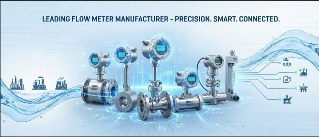
Flow meters are among the most business-critical instruments in any industrial facility. They govern how much chemical is dosed, how accurately custody-transfer volumes are billed, how efficiently energy is managed, and whether regulatory compliance reports hold up to scrutiny. Yet “which flow meter should I buy?” is one of the most frequently asked — and most frequently answered incorrectly — questions in process engineering.
Three technologies dominate industrial liquid and gas metering: ultrasonic flow meters, magnetic (electromagnetic) flow meters, and turbine flow meters. Each rests on a different physical principle; each excels in a specific set of conditions; and each carries a distinct set of trade-offs in accuracy, maintenance burden, and total cost of ownership. The goal of this article is to give facility engineers, procurement managers, and plant operators a practical, data-grounded decision framework — not a vendor brochure.
By the end, you will understand how each technology works at a fundamental level, where each thrives and where it fails, and how to systematically match a meter to your fluid properties, installation constraints, and lifecycle budget. Specific performance data, industry case studies, and application matrixes are included throughout to ground every recommendation in real-world numbers.

Flow measurement instruments on an industrial pipeline network. The wrong technology choice often shows up months after commissioning, in the form of drift, fouling, or process shutdown.
Overview of Flow Meter Technologies
A flow meter is an instrument that quantifies the rate at which a fluid — liquid, gas, or steam — moves through a conduit. Most industrial flow meters measure volumetric flow rate (expressed in m³/h, L/min, or GPM), while a smaller number of technologies measure mass flow rate (kg/h or lb/min) directly. The distinction matters because volumetric measurements must be temperature- and pressure-compensated to calculate mass, whereas mass meters are immune to density changes.
The three technologies covered in this article each occupy a well-defined role in the industrial measurement landscape. Ultrasonic meters use sound waves and require no pipe penetration, making them the only true non-invasive option among the three. Magnetic meters exploit Faraday’s law of electromagnetic induction and are unrivaled for conductive slurries and aggressive liquids. Turbine meters spin a rotor and remain the benchmark for high-accuracy clean-liquid and gas measurement where moving-part wear is manageable.
Quick High-Level Suitability Guide
| Criterion | Ultrasonic | Magnetic (Mag) | Turbine |
|---|---|---|---|
| Fluid type | Clean liquids, non-conductive fluids, gas (transit-time) | Conductive liquids only (≥ 5 µS/cm) | Clean, low-viscosity liquids and gas |
| Typical accuracy | ±0.5 – 1.0% of reading (transit-time) | ±0.2 – 0.5% of reading | ±0.25 – 0.5% of reading |
| Moving parts | None | None | Yes — rotor, bearings |
| Pressure drop | Zero (clamp-on) / Minimal (inline) | Zero (full-bore design) | Moderate (obstruction in pipe) |
| Non-invasive installation | Yes (clamp-on) | No — inline only | No — inline only |
| Abrasive/dirty fluids | Limited (signal scatter) | Excellent (full-bore, no obstruction) | Poor (bearing wear) |
| Relative CAPEX (DN50 inline) | $$ – $$$ | $$ | $ |
How Ultrasonic Flow Meters Work
Ultrasonic flow meters use high-frequency sound waves — typically in the range of 0.5 to 5 MHz — to infer fluid velocity from the behavior of those waves as they travel through a moving medium. There is no physical obstruction inserted into the flow path, which is the defining commercial advantage of the technology.
Transit-Time vs. Doppler: Two Distinct Principles
Transit-time meters (also called time-of-flight meters) place two transducers at a diagonal angle on opposite sides of a pipe. Each transducer alternately transmits and receives. A pulse traveling downstream with the current arrives a tiny fraction of a second sooner than a pulse traveling upstream against the current. That time difference (Δt) is directly proportional to average fluid velocity:
Vf = K × Δt / TL
where Vf is fluid velocity, K is a geometric calibration constant, Δt is the transit-time difference, and TL is the zero-flow transit time. Transit-time technology requires a clean, homogeneous fluid with no significant air bubbles or suspended solids that would scatter the acoustic signal.
Doppler meters emit a continuous ultrasonic beam into the flow. When that beam strikes suspended particles, gas bubbles, or other acoustic reflectors moving with the fluid, it bounces back at a slightly different frequency. The shift in frequency (Δf) is proportional to particle velocity:
V = (f₀ − f₁) × K
Doppler meters therefore require particles or bubbles to function at all — they are purpose-built for dirty, aerated, or slurry-laden fluids. Accuracy is typically ±2–5% of full scale, which suits process monitoring but not custody transfer.
Signal Paths and Installation Considerations
Clamp-on transit-time transducers can be mounted in “V-path” (both transducers on the same side, signal bounces off the opposite wall — suitable for smaller pipes) or “Z-path” (transducers on opposite sides, direct transmission — preferred for large diameters or acoustically challenging pipe materials). Correct acoustic coupling between the transducer face and the pipe wall is critical; a degraded or dried-out couplant gel is one of the most common causes of signal loss in the field.
Standard installation requires 10 pipe diameters (10D) of straight, undisturbed pipe upstream and at least 5D downstream. Elbows, reducers, partially open valves, or pump outlets within those distances distort the flow velocity profile and introduce measurement error. In retrofit situations where straight-run space is limited, multi-path meters (4-path or 8-path configurations) can compensate for some profile distortion.
Common Obstacles and Mitigation
Entrained gas is the most frequent culprit in transit-time signal failure. Even 0.5% air by volume can scatter the acoustic signal enough to trigger a “no signal” alarm. The mitigation is to install the meter at a location where the pipe is guaranteed to be completely full — typically at a low point in the system or on a vertical section with upward flow. Pipe scale and corrosion can attenuate the signal through thick walls; the manufacturer’s signal-strength diagnostic (usually displayed as a percentage) is the first thing to check during troubleshooting.
▶ Video: Ultrasonic Flow Meter Explained — Working Principles (RealPars). An excellent visual walkthrough of transit-time measurement, pipe installation, and signal path geometry.
Pros and Cons of Ultrasonic Flow Meters
Strengths
No moving parts and zero pressure drop (in clamp-on configurations) are the headline advantages. A food-processing plant that switches from a turbine meter to a clamp-on transit-time meter on its water supply line eliminates bearing replacement intervals entirely, while also removing the meter from the hygienic-clean boundary — no wetted components means no contamination risk and no requirement for a process shutdown to pull and inspect the sensor.
Bi-directional measurement is inherent to transit-time technology. The upstream and downstream signals are already being measured; reversing the subtraction order gives reverse flow at no additional hardware cost. This is particularly valuable in tidal or recirculation loops where flow reversal is part of normal operation. Clamp-on installation enables retrofitting to existing pipes without a production halt, cutting commissioning cost dramatically on large-diameter lines — the civil and pipe-cutting cost saved on a single DN600 installation can exceed USD 15,000.
Limitations
Transit-time meters are incompatible with fluids containing significant suspended solids or entrained gas. Wastewater with 5% suspended solids, mining slurries, activated sludge, and pulp-stock suspensions will all scatter the acoustic signal. For those applications, either a Doppler meter (if accuracy requirements are modest) or a magnetic meter (if high accuracy is needed) is the correct choice.
Installation constraints are non-trivial. Pipe material, wall thickness, acoustic velocity of the fluid, and the presence of liners must all be entered correctly into the meter’s configuration. A DN200 HDPE pipe with a rubber liner requires a completely different transducer spacing and coupling approach than a DN200 carbon-steel pipe. Errors in these parameters cause systematic offset errors that are difficult to diagnose in the field without specialist equipment.

Clamp-on transit-time transducers on a large-bore water main. The non-invasive installation eliminates the need for isolation valves or process shutdown during commissioning.
How Magnetic Flow Meters Work
Magnetic flow meters — universally called “mag meters” in the field — operate on Faraday’s law of electromagnetic induction: a conductor moving through a magnetic field generates a voltage proportional to its velocity. In a mag meter, the “conductor” is the conductive fluid; the magnetic field is created by two coils energized from the meter’s power supply; and two electrodes flush-mounted in the pipe wall pick up the tiny induced voltage (typically in the millivolt range) and feed it to the transmitter.
Principle of Operation (Electromagnetic Induction)
The relationship is elegantly linear: double the fluid velocity, and the induced voltage doubles exactly. Because measurement depends only on velocity — not on fluid density, viscosity, or temperature — a properly installed mag meter delivers consistent readings across a remarkably wide operating envelope. A DN100 mag meter measuring municipal water at 2 m/s will give the same ±0.2% accuracy as the same meter measuring 70°C hot process water at 4 m/s, provided the fluid remains conductive.
The pipe section containing the electrodes and coils must be made of non-magnetic material (typically stainless steel or a non-metallic composite) to allow the magnetic field to penetrate without distortion. The interior is lined with an electrical insulator to prevent the induced voltage from short-circuiting through the pipe wall — this liner choice, as discussed later, is one of the most consequential design decisions for chemical applications.
Conductivity Dependence and Material Compatibility
The minimum electrical conductivity threshold for a standard mag meter is approximately 5 µS/cm. Municipal tap water sits at 300–800 µS/cm. Most acids, bases, and industrial brines are 1,000–100,000+ µS/cm. Seawater is ~54,000 µS/cm. All of these work with mag meters without any special consideration.
What does not work: hydrocarbon oils, diesel, petrol, LPG, deionized/ultrapure water below ~1 µS/cm, and organic solvents. If your process fluid falls into these categories, a mag meter is simply not the right technology regardless of price or brand — the physics will not produce a measurable signal.

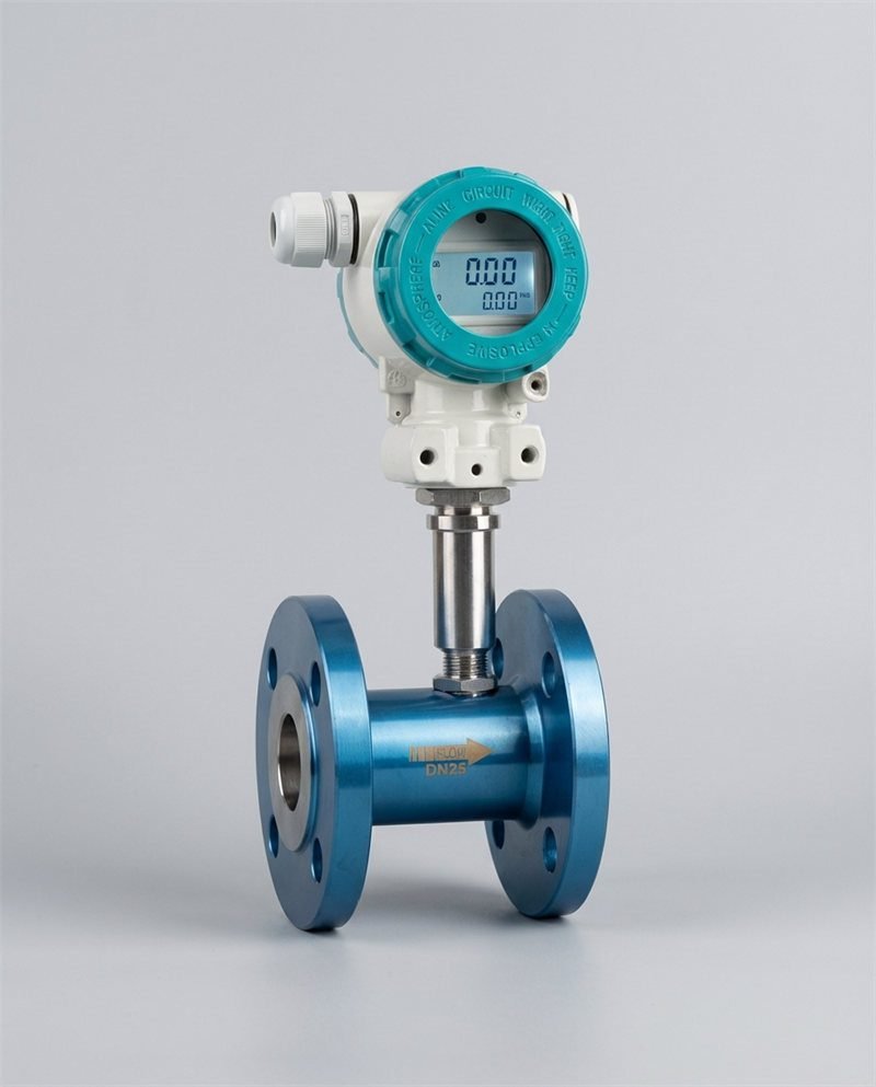
A flanged electromagnetic flow meter on a chemical process line. The full-bore, obstruction-free interior means zero permanent pressure loss — critical for energy-efficient pumping systems.
Installation and Maintenance Considerations
Mag meters are among the most forgiving instruments for straight-pipe requirements: 5D upstream and 2–3D downstream is sufficient for most models, compared with 10–15D for vortex and turbine meters. Some specialized mag meters (notably KROHNE’s ENVIROMAG series) are validated for 0D/0D installation — no straight run required — though these are the exception rather than the rule.
The grounding requirement is frequently overlooked and is the root cause of approximately 50% of all mag meter field failures. Stray electrical currents from variable-frequency drives (VFDs), cathodic protection systems, or welding equipment can interfere with the millivolt-level signal. Proper grounding rings — making direct electrical contact with the process fluid on both flanges — and a dedicated earth conductor (minimum 4 mm² copper) connected to the plant’s earthing grid are non-negotiable on non-metallic or cathodically protected pipelines.
Pros and Cons of Magnetic Flow Meters
Strengths
Wide dynamic range is a defining strength. Most mag meters operate accurately from 0.3 m/s to 10 m/s — a turndown ratio of approximately 33:1 — without any hardware changes. In practice, this means a single DN100 mag meter can handle everything from a trickle-flow condition at night (0.3 m/s, ~85 m³/h) to a peak demand surge in the morning (8 m/s, ~2,260 m³/h) on the same process line.
Zero pressure drop translates directly to pumping energy savings. On a DN200 pipeline pumping 500 m³/h of municipal water, replacing a turbine meter with a mag meter can eliminate a pressure drop of 0.5–1.5 bar, saving 3–9 kW of continuous pumping energy — roughly USD 2,000–5,000 per year at typical industrial electricity tariffs.
Robustness for conductive liquids — including slurries, wastewater, mining pulp, and corrosive acids — is unmatched by any other volumetric technology. A Shandong Province water treatment plant running 34 mag meters on everything from coagulant dosing lines (PTFE liner, Hastelloy electrodes) to filter backwash supply (hard rubber liner, 316L electrodes) reported zero unplanned meter outages over 18 months and a 12% reduction in coagulant consumption attributable to the ±0.2% dosing accuracy. Annual chemical savings: approximately USD 52,000.
Limitations
Not suitable for non-conductive fluids is the hard boundary: no conductivity, no signal. Gases cannot be measured by mag meters under any circumstances. And electrode coating — the gradual buildup of scale, biological film, or chemical deposits on the flush-mounted electrode faces — is the second most common failure mode after grounding, accounting for approximately 20% of field service calls. For fluids prone to scaling (hard water, calcium-rich process streams, biological slurries), self-cleaning electrode designs or higher-frequency AC excitation can reduce but not eliminate coating susceptibility.
Electrode wear in highly abrasive slurry service is a real operational concern. A mining operation running 40% solids-by-weight magnetite slurry through standard 316L electrodes may see visible electrode erosion within 12–18 months. The solution — specifying harder materials like Hastelloy C-276 or adopting KROHNE’s capacitive ENVIROMAG electrode system (where the electrode makes no direct fluid contact) — adds cost at the specification stage but eliminates unplanned replacement in service.
How Turbine Flow Meters Work
A turbine flow meter inserts a multi-bladed rotor into the flow stream. As fluid passes over the blades, it imparts a rotational force on the rotor proportional to the fluid’s linear velocity. A magnetic pickup coil mounted in the meter body generates a pulse for each blade that passes — typically 1 to 8 pulses per rotor revolution. The pulse frequency, therefore, is directly proportional to volumetric flow rate:
Q = f / K-factor
where Q is volumetric flow rate, f is pulse frequency (pulses/second), and the K-factor (pulses/unit volume) is established during factory calibration and is unique to each meter. Because the rotor responds almost instantaneously to changes in flow velocity, turbine meters have excellent dynamic response — they can detect flow fluctuations at frequencies up to several hundred Hz, making them the preferred choice for batch control and flow injection systems where precise cut-off timing is critical.
Positive Displacement vs. Variable-Area Turbine Concepts
It is worth clarifying terminology here. Positive displacement (PD) meters are sometimes loosely grouped with turbine meters but operate on an entirely different principle — they trap fixed volumes of fluid in rotating chambers and count the cycles. True turbine meters infer velocity from rotor speed and convert to volumetric flow via the pipe cross-section. Variable-area (rotameter) meters use gravity to balance a float, providing a visual flow indication rather than an electronic signal. This article focuses on true axial turbine meters, which dominate the precision-liquid and gas-metering segments.
Accuracy Factors and Flow-Range Considerations
A well-calibrated turbine meter for clean liquid service achieves ±0.25% of reading over its linear range, with repeatability better than ±0.05%. However, these figures are only valid within the meter’s specified linear flow range — typically 10:1 turndown. Below approximately 20% of full-scale flow, bearing drag becomes significant relative to the fluid’s driving torque, and the rotor slows faster than the fluid, causing under-reading. This is why turbine meters are not recommended for highly variable-flow applications where low-flow accuracy matters.
Fluid viscosity is the dominant accuracy-limiting variable. Manufacturers’ K-factor calibrations are performed on water (approximately 1 cP at 20°C). As viscosity increases — for oils, glycols, or high-temperature process fluids cooling in the meter — the drag-to-drive ratio changes and the K-factor shifts. Viscosity correction curves or multi-point calibration are necessary for fluids above approximately 5 cP.
Environmental and Installation Factors
Turbine meters require the most demanding installation conditions of the three technologies: 15–20D of straight pipe upstream and 5D downstream. Swirl — the helical velocity component introduced by closely spaced elbows or reducers — is particularly destructive to accuracy because it adds or subtracts from the rotor’s perceived rotational speed. Flow straighteners or flow conditioners installed upstream can reduce the straight-run requirement to approximately 10D in constrained installations.

A turbine flow meter with its rotor assembly visible. The multi-bladed rotor must spin freely on low-friction bearings — clean, non-abrasive fluid and correct viscosity matching are prerequisites for achieving ±0.25% accuracy.
Pros and Cons of Turbine Flow Meters
Strengths
High accuracy on clean liquids and gas is the turbine meter’s defining commercial proposition. In custody-transfer applications for petroleum, LPG, and refined products — where even a 0.05% measurement error translates to significant financial loss over millions of barrels — turbine meters remain the benchmark technology. A properly calibrated turbine meter for petroleum service maintains ±0.15% of reading over its linear range, which no ultrasonic or magnetic meter currently matches on a consistent, long-term basis without frequent recalibration.
Fast dynamic response makes turbine meters the standard tool for batch controllers and piston filling machines where the “meter-stop” command must account for the fluid still in the pipe at the moment the valve closes. Response times of 20–50 ms are routinely achievable with a rotor-pulse-based turbine meter — compared with 100–500 ms for the averaging window of most electronic ultrasonic or mag meter transmitters.
Low initial cost relative to ultrasonic and magnetic meters is a practical advantage in large-scale installations. A DN25 turbine meter for clean water or chemical service typically costs USD 300–800, versus USD 800–1,500 for a comparable inline mag meter and USD 1,000–2,500 for an ultrasonic meter of equivalent accuracy.
Limitations
Moving parts are the fundamental vulnerability. Rotor bearings wear under the continuous mechanical load of spinning in a fluid stream, and wear rate accelerates with fluid velocity, viscosity, and any particulate content. In a petroleum product pipeline running at 3 m/s with nominally clean fluid, bearing replacement is typically required every 18–36 months. In a water system with minor sand content, the same bearing may need replacement every 6–9 months — and each replacement requires isolating and draining the line.
Fouling risk is acute in any fluid containing biological growth potential, mineral scaling tendency, or polymer residues. A biofilm even 0.3 mm thick on a rotor blade changes the blade profile enough to shift the K-factor by 0.5–2% — an invisible error that accumulates between calibration checks. Viscosity sensitivity means that a turbine meter calibrated on water at 20°C will give systematic errors when used on a fluid at a different temperature and viscosity without appropriate correction.
Factors to Consider When Choosing a Flow Meter
Fluid Properties: Conductivity, Viscosity, and Particulates
The fluid is the starting point — every other selection criterion is secondary. Before specifying any meter, document the following for your process fluid: electrical conductivity (µS/cm), viscosity at operating temperature (cP or mPa·s), density, presence and concentration of suspended solids or gas bubbles, chemical aggressiveness (pH, oxidizing potential, concentration of halides), temperature range (minimum, maximum, and typical), and pressure range. This fluid profile immediately eliminates certain technologies and narrows the field.
Required Accuracy, Flow Range, and Installation Constraints
Define your accuracy requirement in concrete business terms, not just as a percentage. A ±1% error on a 100 m³/h water supply line means 1 m³/h of undetected discrepancy — probably acceptable for a general water balance. The same ±1% error on a USD 120/tonne chemical feed at 10 m³/h represents USD 1,200/h in measurement uncertainty — emphatically not acceptable for custody transfer or process yield control. Once the acceptable monetary error is defined, the accuracy requirement follows naturally.
Flow range and turndown ratio deserve specific attention. If your process regularly operates at both 5% and 100% of maximum design flow, you need a meter with at least 20:1 turndown — which favors mag meters and transit-time ultrasonic meters over turbine meters (typically 10:1).
Maintenance, Lifecycle Cost, and Downtime Implications
Purchase price accounts for only 30–40% of a flow meter’s 10-year total cost of ownership (TCO). Calibration, spare parts, unplanned downtime, and decommissioning for maintenance make up the remainder. For a turbine meter on a petroleum line, the bearing replacement cost over 10 years (assuming 3 replacements at USD 400–600 each, plus 4–8 hours of process downtime at USD 500–1,500/hour) can exceed the original purchase price. A mag meter on the same line has no moving parts to replace and can often be verified in-situ using a transmitter self-diagnostic — avoiding the shutdown entirely.
Industry Applications and Best Use Cases
Matching a flow meter technology to an industry and application is one of the most reliable shortcuts in the selection process. The following guidance reflects actual practice across thousands of installations — not theoretical capability, but the technology that experienced engineers actually specify when they have full information.
Ultrasonic: Large Meters, Dirty or Clean Liquids, Non-Invasive Options
Transit-time ultrasonic meters are the standard choice for large-bore (DN200 and above) clean water distribution lines, where the cost advantage of clamp-on installation is most pronounced. A DN600 water main at a municipal utility: the cost of cutting the pipe, installing a flanged inline meter, and restoring service easily exceeds USD 30,000. Clamping two transducers onto the existing pipe takes one technician half a day.
In the oil and gas sector, multi-path transit-time meters (4-path or 8-path configurations per AGA-9 standards for gas, or OIML R117 for liquid) are increasingly displacing turbine meters for fiscal gas metering above DN150, because they eliminate the mechanical wear that requires custody-transfer-grade recalibration every 6–12 months. A major North Sea operator reported that switching from turbine to 4-path ultrasonic meters on 40 fiscal gas measurement stations reduced annual calibration costs by approximately USD 1.8 million.
Doppler ultrasonic meters cover the wastewater monitoring segment — where transit-time meters fail — providing 2–5% process monitoring accuracy for activated sludge, raw sewage influent, and storm-water overflow measurement. For this segment, teams at Jade Ant Instruments recommend reviewing the fluid’s solids concentration and particle size distribution before finalizing the transducer specification.
Magnetic: Conductive Liquids, Slurry Tolerance, Sanitary Processes
Mag meters are the default specification for water treatment, wastewater, chemical dosing, mining, pulp and paper, and food and beverage whenever the fluid is conductive. The absence of any pipe obstruction is decisive in slurry service: a turbine meter would clog within hours on a 25% solids-by-weight paper-pulp suspension; a mag meter runs indefinitely with no wear.
Sanitary mag meters with PFA liners, polished stainless steel bodies, and hygienic flanged or tri-clamp connections are the standard in pharmaceutical API production, dairy processing, and beverage blending — applications where every surface in contact with product must be cleanable in place (CIP), sterilizable in place (SIP), and free of crevices that harbor contamination. Jade Ant Instruments’ electromagnetic flow meter selection guide covers liner and electrode compatibility for over 40 chemical compounds, including common food-grade acids and alkaline CIP chemicals.
Turbine: Custody Transfer, Clean Liquids, Stringent Accuracy Needs
Petroleum custody transfer — the precise measurement of oil, refined products, LPG, and natural gas at financial transaction boundaries — is where turbine meters have the deepest track record. API MPMS Chapter 5 and AGA-7 specify turbine meters as approved technologies for fiscal metering. A refinery delivering 10,000 barrels of crude oil per hour needs sub-0.2% accuracy: a 0.1% meter error at USD 80/barrel represents USD 8,000 per hour of financial exposure.
Chemical batch dispensing is another turbine stronghold. The fast pulse-based output of a turbine meter integrates perfectly with a batch controller’s totalizer function, enabling accurate cut-off to within ±0.1% of a target batch volume — critical for blending high-value specialty chemicals or pharmaceutical excipients where a 1% excess of one component can fail an entire batch worth USD 50,000+.
Technology Comparison: Data at a Glance
Head-to-Head Performance Comparison Table
| Parameter | Ultrasonic (Transit-Time) | Magnetic (Electromagnetic) | Turbine |
|---|---|---|---|
| Operating principle | Transit-time difference of sound pulses | Faraday’s law (induced voltage) | Rotor pulse frequency |
| Best accuracy (inline) | ±0.5% of reading | ±0.2% of reading | ±0.25% of reading |
| Repeatability | ±0.1 – 0.2% | ±0.1% | ±0.02 – 0.05% |
| Typical turndown ratio | 100:1 (multi-path) | 33:1 standard | 10:1 |
| Pressure drop | None (clamp-on) / ~0.01 bar (inline) | None (full-bore) | Moderate: 0.1–0.8 bar at full flow |
| Minimum conductivity | None required | ≥ 5 µS/cm | None required |
| Gas measurement | Yes (specialized transducers per AGA-9) | No | Yes (AGA-7 for natural gas) |
| Moving parts | None | None | Yes — rotor, bearings |
| Abrasive/slurry tolerance | Low (signal scatter) | Excellent (full-bore, ceramic liner available) | Very poor (rapid bearing wear) |
| Non-invasive installation | Yes (clamp-on) | No | No |
| Viscosity sensitivity | Moderate (density/SOS correction needed above 5 cP) | None (velocity only) | High (K-factor shifts above ~5 cP) |
| Upstream straight run required | 10D upstream / 5D downstream | 5D upstream / 2–3D downstream | 15–20D upstream / 5D downstream |
| Calibration interval (typical) | 3–5 years (in-situ diagnostic capable) | 2–3 years (in-situ diagnostic capable) | 1–2 years (mechanical wear requires more frequent checks) |
| Typical CAPEX (DN50 inline) | USD 1,000 – 3,500 | USD 800 – 4,500 | USD 300 – 1,200 |
| 10-year TCO estimate (DN50) | USD 6,000 – 10,000 | USD 7,000 – 12,000 | USD 5,500 – 14,000 (depending on bearing wear rate) |
Accuracy Comparison by Technology (Bar Chart)
Best Achievable Accuracy — Inline Meters (Lower % = Better)
Source: Manufacturer datasheets and industry benchmarks. Accuracy figures apply to specified operating conditions and flow ranges only.
Typical Industry Application by Technology (Pie Chart)
Primary Industrial Application Distribution by Flow Meter Technology
Flow Meter
Applications
- Water & Wastewater — 35% (Predominantly Magnetic)
- Oil & Gas — 25% (Predominantly Turbine + Ultrasonic)
- Chemical Processing — 20% (Predominantly Magnetic)
- Large-Bore Water Mains — 12% (Predominantly Ultrasonic)
- HVAC & Utilities — 5% (Ultrasonic / Turbine)
- Other Industries — 3%
Approximate distribution based on global flow meter market segment data (Fortune Business Insights, 2025). Within each segment, multiple technologies compete; dominant technology shown.
Maintenance, Calibration, and Longevity
Maintenance requirements are where the TCO differences between the three technologies become most visible. Two facilities that pay the same purchase price for different technologies will face dramatically different operational cost profiles over a 10-year horizon.
Calibration Routines and Drift Management
The industry-standard calibration interval is every 2–3 years for general process service and annually for custody-transfer or regulatory compliance points. However, this interval is based on historical practice and does not account for the in-situ diagnostic capabilities of modern meters.
Endress+Hauser’s Heartbeat Technology and Siemens’ SENSORPROM can generate a traceable verification certificate without interrupting the process — confirming that the sensor and transmitter are performing within specification and, if they are, justifying extension of the calibration interval to 5 or even 7 years under ISO 9001 risk-based quality management. One European pharmaceutical plant extended its mag meter calibration interval from 12 to 36 months using in-situ Heartbeat verification, saving approximately EUR 12,000 per year in external calibration costs across 18 measurement points.
Turbine meters, with their mechanically wearing rotors, do not generally support in-situ verification to the same standard. The rotor K-factor shifts progressively with bearing wear, so calibration requires either a calibration rig with a reference standard or removal of the meter from service — an operational constraint that does not apply to mag or ultrasonic meters.
Common Wear Parts and Replacement Timelines
| Component | Ultrasonic | Magnetic | Turbine | Typical Replacement Interval |
|---|---|---|---|---|
| Rotor / Bearings | N/A | N/A | Required | 18 – 36 months (clean liquid); 6 – 12 months (moderate contamination) |
| Transducer / Couplant | Inspect every 2–3 years | N/A | N/A | Couplant refresh: 3–5 years |
| Electrode cleaning / replacement | N/A | Annual inspection | N/A | Cleaning: as needed; replacement: 5–15 years (material dependent) |
| Liner replacement | N/A | Conditional | N/A | Hard rubber (municipal water): 15–20 years; PU (abrasive slurry): 5–8 years |
| Transmitter electronics | Inspect every 5–7 years | Inspect every 5–7 years | Inspect every 3–5 years | Replacement: 10–15 years (capacitor aging, display degradation) |
| Intervals are indicative and vary by process conditions, fluid aggressiveness, and manufacturer model. Always refer to the specific product’s maintenance schedule. | ||||
Best Practices for Reliability and Uptime
Regardless of technology, installation quality at commissioning determines more of the long-term reliability outcome than the choice of brand. Verifying pipe-full conditions before start-up, confirming grounding continuity (for mag meters), checking transducer coupling signal strength (for ultrasonic), and performing a zero-point verification (flowing the meter at zero flow to confirm the transmitter offset is within specification) are the four most impactful commissioning checks — and the four most frequently skipped.
For magnetic flow meter maintenance specifically, a structured annual inspection protocol — checking electrode resistance, verifying coil resistance, confirming signal cable integrity, and reviewing transmitter diagnostics — catches the majority of developing faults before they cause a measurement failure.
Safety, Compliance, and Certifications
Standards to Consider (ISO, API, AGA Guidelines)
Industrial flow measurement operates within a layered framework of international and regional standards. The most relevant for the three technologies covered in this article are:
- ISO 4064 (Water meters for cold potable water and hot water) — governs accuracy class, installation, and performance for municipal water billing meters, primarily magnetic and ultrasonic.
- API MPMS Chapter 5 (Turbine Meters) and AGA-7 (Measurement of Natural Gas by Turbine Meters) — the primary custody-transfer standards for turbine meters in petroleum and gas service.
- AGA-9 (Measurement of Natural Gas by Multipath Ultrasonic Meters) — the authoritative standard for ultrasonic gas meters in fiscal metering, requiring a minimum of 4 acoustic paths and factory calibration traceable to national standards.
- OIML R117 (Dynamic Measuring Systems for Liquids) — the European-framework metrology standard for liquid custody-transfer meters, used for both mag meters and turbine meters in EU applications.
- ISO 9001 — the quality management standard that underpins manufacturing and calibration traceability. ISO 9001-certified manufacturers, including Jade Ant Instruments, provide calibration certificates traceable to national metrology standards.
Electrical and Installation Safety Notes
Flow meters installed in hazardous area classifications (Zone 0, 1, 2 for gas; Zone 20, 21, 22 for dust per IEC 60079) require ATEX (EU) or IECEx (international) certification for the transmitter and, in intrinsically safe systems, the sensor coils and signal cables. Most major manufacturers offer Ex-certified variants of their flagship products. Always verify the specific zone classification of the installation point against the meter’s Ex marking — using an Ex d (explosion-proof) transmitter in an Ex ia (intrinsically safe) system, or vice versa, is an electrical safety violation regardless of the certification label.
Documentation and Traceability for Audits
Regulatory audits — whether for water utility billing compliance, pharmaceutical GMP validation, or custody-transfer fiscal metering — require a complete document package: original factory calibration certificate, installation record, commissioning test report, and periodic re-calibration records. In-situ verification tools (Heartbeat, SENSORPROM) generate traceable PDF reports that satisfy these requirements without a meter pull and send. For plants subject to 21 CFR Part 11 (FDA electronic records) or EU GMP Annex 11, electronic audit trails with time-stamped operator authentication are mandatory — a feature available on most modern smart transmitters via HART or fieldbus protocol.

A modern SCADA control room receiving real-time flow measurement data. Digital communication protocols (HART, Modbus, Profibus, Ethernet APL) transform individual meters into networked measurement assets with full audit trails.
Cost of Ownership and Total Cost of Implementation
CAPEX vs. OPEX Considerations
The turbine meter’s low purchase price is frequently the decisive factor in initial budgeting — and frequently the reason a facility ends up spending more over 10 years than it would have with a higher-CAPEX alternative. The reasoning is straightforward: a DN50 turbine meter costing USD 600 on a petroleum product line will likely require at least 3 bearing replacements over 10 years (USD 1,800 in parts), plus 3 calibration pulls at USD 800–1,200 each (USD 2,400–3,600 in calibration), plus 24–48 hours of process downtime across those events (USD 3,600–14,400 at USD 150–300/hour for a mid-scale facility). The total 10-year cost: USD 8,400–19,800 — against a purchase price of USD 600.
Long-Term Maintenance and Calibration Costs
10-Year Total Cost of Ownership — DN50 Process Line (USD, Indicative)
Indicative estimates. Includes CAPEX, installation (USD 800), calibration (3 intervals), wear parts, spare transmitter, and estimated downtime cost. Actual figures vary by application, fluid, and maintenance strategy.
Replacement Cycles and Downtime Impact
The financial weight of downtime is the most frequently underestimated element of TCO. In a continuous chemical process running at USD 5,000/hour gross margin, a 4-hour meter replacement event costs USD 20,000 in lost production — dwarfing any difference in purchase price between a USD 900 turbine meter and a USD 2,500 mag meter with no moving parts. Facilities with high-value continuous processes should always model downtime cost explicitly in their TCO comparison. The five-factor flow meter selection framework from Jade Ant Instruments provides a structured calculation method for building this model.
📖 Quick Glossary of Key Terms
- Transit-time difference (Δt)
- The tiny difference in travel time between an ultrasonic pulse sent downstream (with flow) versus upstream (against flow); the core measurement signal in transit-time ultrasonic meters.
- Faraday’s law of electromagnetic induction
- The physics principle that a conductor (here: conductive liquid) moving through a magnetic field generates a voltage proportional to its velocity — the operating principle of all magnetic flow meters.
- K-factor
- The calibration constant of a turbine meter, expressed as pulses per unit volume (e.g., pulses/litre). Established at factory calibration; shifts with bearing wear or viscosity changes.
- Turndown ratio
- The ratio of maximum to minimum measurable flow rate at which the meter meets its accuracy specification. A 33:1 turndown means the meter is accurate from 3% to 100% of its rated maximum flow.
- Total Cost of Ownership (TCO)
- The sum of purchase price, installation, calibration, maintenance, spare parts, and downtime cost over the meter’s operating life — typically modeled over 10 years.
- Liner
- The non-conductive, chemically resistant coating on the inside bore of a magnetic flow meter that insulates the pipe wall from the induced electrical signal and protects the metal body from the process fluid.
- ATEX / IECEx
- Certification schemes (European and international, respectively) that validate the safety of electrical equipment for use in potentially explosive atmospheres (hazardous area classification).
A Practical Decision Framework
The headline answer to “which flow meter is best for your facility?” is: the one whose physical operating principle matches the properties of your process fluid, whose installation requirements fit your available space, and whose lifecycle cost structure aligns with your operational priorities. There is no universally superior technology — there is only the right technology for each specific application.
Choose ultrasonic when you need non-invasive installation on large-bore pipes, when retrofitting without a process shutdown is a business requirement, when your fluid is non-conductive (ruling out mag meters), or when fiscal gas metering above DN150 demands multi-path AGA-9 compliance with reduced mechanical maintenance.
Choose magnetic when your fluid is conductive (which covers the majority of aqueous industrial processes), when slurries, abrasive fluids, or dirty water are involved, when zero pressure drop and wide dynamic range are priorities, and when sanitary CIP/SIP compatibility is required in food, pharmaceutical, or biotechnology applications.
Choose turbine when the highest accuracy on clean, low-viscosity liquids or gas is the overriding requirement, when custody-transfer billing under API or AGA standards is involved, when fast dynamic response for batch control is needed, and when the process conditions guarantee low wear rates that keep the TCO competitive with no-moving-parts alternatives.
For pilot validation, always test on your actual process fluid at your actual operating conditions before full-scale procurement. Vendor-supplied demo meters are available from most reputable manufacturers for this purpose. And for facilities specifying multiple meters across a new plant — where the technology mix decision multiplies in financial impact — a structured vendor consultation covering your complete fluid portfolio, installation map, and lifecycle expectations is the most cost-effective investment you can make before issuing purchase orders.
Need Help Matching the Right Flow Meter to Your Process?
Jade Ant Instruments manufactures ISO 9001-certified electromagnetic, turbine, ultrasonic, vortex, and thermal flow meters for industrial applications worldwide. Our engineering team provides free technical consultation and sizing support.
Frequently Asked Questions
Click any question to expand the answer.
Which flow meter is best for dirty fluids or wastewater?
Magnetic flow meters are the dominant choice for dirty fluids — wastewater, sewage, mining slurries, paper pulp, and any fluid with suspended solids above approximately 1% by volume. The full-bore, obstruction-free design means solids pass through without clogging, and the correct liner material (hard rubber or polyurethane for abrasive applications, PTFE for corrosive media) protects the instrument body from chemical attack. Mag meters can handle solids concentrations exceeding 40% by weight in well-engineered mining installations. Transit-time ultrasonic meters are not suitable for dirty fluids because suspended solids scatter the acoustic signal; Doppler ultrasonic meters offer an alternative for dirty fluid monitoring where ±2–5% accuracy is sufficient. Turbine meters are generally unsuitable for dirty fluids — particulates damage the rotor bearings rapidly.
Can a single flow meter measure multiple fluid types across different shifts or batches?
In principle, yes — but with important caveats. A magnetic flow meter can measure any conductive fluid without recalibration, as long as the liner and electrode materials are chemically compatible with all fluids in the rotation. A transit-time ultrasonic meter can handle multiple clean fluids, but if the fluids have significantly different speeds of sound (e.g., switching between water and a dense glycol solution), the meter must be reconfigured with the correct fluid acoustic properties to maintain accuracy. A turbine meter calibrated on water will give systematic errors when used on a fluid with a different viscosity, and viscosity correction coefficients must be applied. For multi-fluid applications, verify chemical compatibility for every fluid in the rotation — not just the primary fluid — and confirm with the manufacturer that the configuration approach is validated.
How often should calibration be performed for each flow meter technology?
For general process service, the industry standard is every 2–3 years for magnetic and ultrasonic meters and every 1–2 years for turbine meters. For custody-transfer or regulatory-compliance points, annual calibration is typical for all technologies. However, modern magnetic and ultrasonic meters equipped with in-situ diagnostic systems (Endress+Hauser Heartbeat Technology, Siemens SENSORPROM) can generate traceable verification records without removing the meter from service, enabling risk-based extension of calibration intervals to 5 years or more under ISO 9001 quality management frameworks. The Fluke flowmeter calibration best practices guide provides detailed guidance on setting calibration frequencies based on measurement criticality and historical drift data.
What is the minimum straight-pipe run required for each flow meter type?
Turbine meters require the longest straight run: 15–20 pipe diameters (D) upstream and 5D downstream, because the rotor is highly sensitive to swirl and asymmetric flow profiles introduced by upstream fittings. Ultrasonic transit-time meters typically require 10D upstream and 5D downstream, though multi-path configurations can tolerate somewhat shorter runs. Magnetic flow meters are the most forgiving: 5D upstream and 2–3D downstream is standard, and some validated models (notably KROHNE’s ENVIROMAG with Weymouth method) claim 0D/0D for specific custody-transfer-grade applications. In all cases, refer to the specific product’s installation manual — generic rules are starting points, not substitutes for model-specific guidance.
Can ultrasonic flow meters measure gas flow, or only liquids?
Transit-time ultrasonic meters can measure gas flow, but require specialized transducers designed for the much lower acoustic impedance and density of gases compared to liquids. Multi-path ultrasonic gas meters operating under AGA-9 are widely used in natural gas fiscal metering and are increasingly displacing turbine meters in high-pressure gas pipelines above DN150 due to their lower maintenance requirements. Doppler ultrasonic meters are generally not used for gas measurement because clean gas streams lack the acoustic reflectors (particles or bubbles) that the Doppler principle requires. Magnetic flow meters cannot measure gas under any circumstances.
What fluid conductivity is required for a magnetic flow meter to work?
Standard commercial magnetic flow meters require a minimum fluid conductivity of approximately 5 µS/cm. This threshold is met comfortably by municipal tap water (300–800 µS/cm), most acids and bases (1,000–100,000+ µS/cm), seawater (~54,000 µS/cm), and most aqueous industrial process fluids. Fluids that fall below this threshold — and therefore cannot be measured by a mag meter — include hydrocarbon oils and fuels, deionized or ultrapure water below ~1 µS/cm, liquefied gases, and most organic solvents. A simple handheld conductivity meter (under USD 50) can verify your fluid’s conductivity on-site before specifying. Some specialized mag meters claim operability down to 0.5 µS/cm for specific ultrapure-water applications, but these are niche products at a significant cost premium.
What is the difference between a magnetic flow meter and an electromagnetic flow meter?
There is no functional difference — “magnetic flow meter,” “electromagnetic flow meter,” and “mag meter” are three terms for exactly the same instrument. All three names refer to a volumetric flow meter that operates on Faraday’s law of electromagnetic induction, using a magnetic field to induce a voltage in a flowing conductive liquid, which is then measured by flush-mounted electrodes. The term “electromagnetic flow meter” or “EMF” is more common in technical and academic literature; “magnetic flow meter” and “mag meter” are more common in field use. Manufacturers and suppliers, including Jade Ant Instruments, use all three interchangeably in their product literature.
Why is my flow meter reading inaccurate after working correctly for years?
The most likely causes differ by technology. For magnetic flow meters: electrode coating (scale, biofilm, or chemical deposit on the electrode face) is the most common culprit for a gradual drift toward lower readings; grounding degradation (corrosion of grounding rings or a broken earth conductor) causes erratic, high-noise readings. For turbine meters: bearing wear is the primary cause of a gradual K-factor shift, typically producing under-reading at low flows and over-reading at high flows; rotor fouling or partial blade damage produces erratic readings. For ultrasonic meters: degraded transducer couplant (gel dried out or washed away) causes declining signal strength; pipe wall scale buildup at the transducer location attenuates the signal. In all three cases, the first diagnostic step is to review the transmitter’s internal diagnostic outputs — signal strength, noise level, and diagnostic flags — before any physical inspection.
Are turbine flow meters suitable for steam or high-temperature applications?
Standard liquid turbine meters are typically rated to 120–150°C maximum fluid temperature, which covers hot water and many process liquids but not steam. High-temperature turbine meters with ceramic or high-temperature alloy bearings extend the range to approximately 200°C for liquid service. Gas turbine meters for natural gas service are generally limited to 60–80°C. For steam flow measurement, vortex flow meters are the standard choice — they have no moving parts, tolerate steam temperatures up to 300°C+, and are available in configurations that simultaneously measure flow rate and energy (MJ/h) using an integrated temperature and pressure sensor. Magnetic flow meters cannot measure steam or any gas. Ultrasonic meters can measure hot liquids but require transducers rated for the specific temperature range.
How do I select between ultrasonic, magnetic, and turbine meters for a new facility with multiple fluid types?
The most systematic approach is a fluid-by-fluid decision matrix. For each measurement point: (1) Document the fluid properties — conductivity, viscosity, solids content, chemical aggressiveness, temperature. (2) Apply the exclusion criteria — non-conductive fluids rule out mag meters; fluids with significant solids rule out turbine and transit-time ultrasonic; gas rules out mag meters. (3) Apply accuracy requirements — custody transfer or fiscal metering favors mag meters (±0.2%) or turbine meters (±0.25%); process monitoring tolerates ±1% or higher. (4) Apply installation constraints — limited straight run favors mag meters; retrofit without shutdown favors clamp-on ultrasonic. (5) Model 10-year TCO including downtime cost for each candidate technology. In multi-meter facilities, standardizing on one or two technologies wherever application requirements allow reduces spare parts inventory and operator training cost. For large-scale facility projects, the Jade Ant Instruments supplier selection guide and Engineering ToolBox flow meter comparison resource provide complementary decision frameworks.