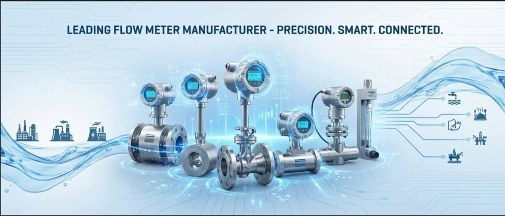
The global ultrasonic flow meter market reached USD 2.08 billion in 2025 and is forecast to hit USD 3.56 billion by 2034 — not because the technology is new, but because industries keep discovering how much money they leave on the table with legacy mechanical meters. A 1% measurement error on a municipal water network losing 18% of treated water to unmetered leakage represents millions of dollars in annual revenue loss. This guide explains the physics behind ultrasonic measurement — transit-time and Doppler shift — clearly enough that your sales and technical teams can explain it to any client, regardless of their background.
1. Fundamentals of Sound Waves and Acoustic Principles
What Are Sound Waves and How Do They Behave in Fluids?
A sound wave is a mechanical pressure disturbance — a series of compressions and rarefactions — that propagates through a medium by transferring energy from particle to particle. Unlike electromagnetic waves (light, radio), sound waves cannot travel through a vacuum. They need a medium: a solid, liquid, or gas.
Three properties define any sound wave. Frequency (measured in Hertz, Hz) is the number of compression cycles per second. Human hearing covers roughly 20 Hz to 20 kHz. Ultrasonic flow meters operate between 0.5 MHz and 10 MHz — far above hearing range, which is why they are called “ultrasonic.” Wavelength is the physical distance from one compression peak to the next; it shortens as frequency increases. Amplitude is the intensity of the pressure variation, which determines signal strength and how far the wave can travel before being absorbed.
In fluids, sound propagates as longitudinal waves — the particles vibrate parallel to the direction of wave travel, creating alternating zones of high and low pressure. The speed at which this pressure wave travels through the fluid is what makes ultrasonic flow measurement possible.
Speed of Sound Variations in Liquids and Gases
Sound travels through water at approximately 1,480 m/s at 20°C — nearly four times faster than through air (343 m/s at 20°C) — because water molecules are more densely packed and can transfer pressure more efficiently. This matters enormously for flow meter design: the transit-time difference that the meter must measure at a typical flow velocity of 1–3 m/s is in the range of microseconds to nanoseconds, requiring extremely precise electronic timing circuits.

Flow measurement instrumentation in a water treatment facility. The speed of sound through the process fluid — which varies with temperature, pressure, and fluid composition — is the physical variable that every ultrasonic flow meter exploits to determine flow velocity.
Key Acoustic Properties Relevant to Flow Measurement
Acoustic Impedance and Its Importance
Acoustic impedance (Z) is the resistance a medium presents to the propagation of a sound wave. It is defined as the product of the medium’s density (ρ) and the speed of sound (c):
When a sound wave crosses a boundary between two materials with different acoustic impedances — say, the steel pipe wall and the water inside — a fraction of the energy is reflected back and a fraction is transmitted forward. The greater the impedance mismatch, the more energy is reflected and the less reaches the receiving transducer. This is why a clamp-on meter cannot work on a pipe with an internal rubber lining: the air gap between the steel and the rubber creates a near-total acoustic reflection, effectively blocking the signal.
Temperature and Pressure Effects on Sound Propagation
Temperature raises the speed of sound in liquids — water at 80°C transmits sound at approximately 1,550 m/s versus 1,480 m/s at 20°C, a difference of about 5%. In gases, the speed of sound is proportional to the square root of absolute temperature: a natural gas line at 60°C versus 20°C carries sound roughly 7% faster. Without active compensation for these changes, a meter calibrated at one temperature will give systematic errors at another. All quality ultrasonic meters address this with built-in temperature sensors and correction algorithms.
Pressure has a smaller but non-negligible effect on liquid measurement (liquids are nearly incompressible), but a significant effect on gas measurement: higher pressure increases gas density, changing both sound speed and acoustic impedance. Gas ultrasonic meters used for custody transfer include pressure transmitter inputs and real gas equation-of-state calculations to correct measured volumes to standard conditions.
2. Introduction to Ultrasonic Flow Meters
The Advantages of Ultrasonic Technology Over Traditional Methods
Turbine meters and orifice plates — the workhorses of industrial flow measurement for most of the 20th century — share a fundamental vulnerability: they involve mechanical contact with the fluid. Turbine rotors wear. Orifice plate edges erode. Bearing seals fail. Every maintenance event means a process shutdown, a calibration verification, and direct contact with whatever fluid the line carries. In a pharmaceutical WFI loop, a chemical acid line, or a cryogenic system, “contact with the fluid” ranges from inconvenient to hazardous to impossible.
Ultrasonic flow meters eliminate this problem class entirely. The measurement is acoustic — sound waves passing through the pipe wall and fluid, with transducers that in clamp-on configurations never touch the process fluid at all. No rotating parts. No differential pressure ports that can plug. No wetted seals that degrade in aggressive media.
✔ Ultrasonic Advantages
- No moving parts → no mechanical wear
- Zero pressure drop across the meter
- Non-invasive clamp-on installation possible
- Bidirectional measurement as standard
- Covers DN15 to DN6000+ pipe sizes
- 10–15+ year operational lifespan
- Compatible with corrosive and pure fluids
⚠ Where to Apply Carefully
- Aerated or multiphase fluids (transit-time)
- Very low acoustic impedance gases (need specialist design)
- Heavily corroded or lined pipe walls
- Extreme high-temperature above 200°C (needs HT transducers)
- Custody transfer: requires inline multi-path certification
- Fluids below required particle threshold (Doppler)
When and Why to Choose Ultrasonic Flow Meters
Comparison with Magnetic and Turbine Flow Meters
The choice between ultrasonic, magnetic, and turbine meters comes down to three variables: fluid conductivity, required accuracy, and installation constraints. Electromagnetic (mag) flow meters achieve excellent accuracy (±0.2–0.5%) but require the fluid to be electrically conductive — ruling them out for hydrocarbons, deionised water, and most gases. Turbine meters offer ±0.5–1.0% accuracy but have mechanical rotors that wear over time, require clean fluids without suspended solids, and create a modest pressure drop. Ultrasonic meters cover the widest application range: they work on conductive and non-conductive fluids, require no process contact in clamp-on form, and handle pipe sizes that make turbine or mag meters prohibitively expensive at large diameters.
Table 1: Ultrasonic vs. Electromagnetic vs. Turbine Flow Meters — Key Comparison
| Criterion | Ultrasonic (Transit-Time) | Electromagnetic (Mag) | التوربينات |
|---|---|---|---|
| Fluid conductivity required? | لا يوجد | Yes (min. 5 µS/cm) | لا يوجد |
| Fluid must be clean? | Yes (transit-time) / No (Doppler) | Tolerates light solids | Yes — solids damage rotor |
| Moving parts? | لا شيء | لا شيء | Yes — rotor and bearings |
| Pressure drop | Zero (clamp-on/inline) | Negligible | Moderate (obstruction) |
| Typical accuracy | ±0.15–2% (by type) | ±0.2–0.5% | ±0.5–1.0% |
| Max pipe size (practical) | DN6000+ (insertion) | DN3000 | DN600 (cost prohibitive above) |
| Maintenance frequency | Low (no wear parts) | Low (electrode cleaning) | Moderate–High (bearing wear) |
| Non-invasive option? | Yes — clamp-on | لا يوجد | لا يوجد |
3. The Transit-Time Principle Explained
How Transit-Time Measurement Works
Transit-time measurement exploits one of the most elegant physical relationships in flow instrumentation: when a fluid is moving through a pipe, sound travels faster in the direction of flow and slower against it. The meter does not directly measure the speed of sound — it measures the difference between the two travel times, which is directly proportional to the fluid velocity.
Think of it as two swimmers crossing the same river. One swims with the current, one against it. The one swimming downstream crosses faster. The difference in their crossing times tells you how fast the current is flowing — without needing to know anything about each swimmer’s individual speed.
Vfluid = (L / 2 cos θ) × (Δt / tup × tdown) L = path length between transducers | θ = transducer angle relative to pipe axis | Δt = transit-time difference | Vfluid = average fluid velocity
Volumetric flow rate (Q) is then calculated by multiplying the fluid velocity by the pipe’s cross-sectional area (A):
Step-by-Step Breakdown of the Transit-Time Process
Understanding Signal Propagation
▲ A clear, professionally produced explanation of how ultrasonic flow meters work — covering piezoelectric transducer operation, transit-time and Doppler principles, and key application differences. Ideal reference material for distributor technical training sessions.
Velocity Calculation and Conversion to Flow Rate
The raw transit-time measurement contains the average velocity along the acoustic path — not the average velocity across the full pipe cross-section. In real pipes, the fluid velocity profile is not uniform: it is faster at the centre than at the walls (parabolic in laminar flow, flatter in turbulent flow). A correction factor — the profile factor K — adjusts for this, and its value is programmed into the meter based on the pipe’s Reynolds number (the ratio of inertial to viscous forces in the flow).
Multi-path meters address the profile issue more rigorously by using 2, 4, or even 8 acoustic chords at different positions across the pipe diameter. Each chord samples a different radial position; a numerical integration (typically using Gaussian or Gauss-Jacobi quadrature weighting) across all paths yields a far more accurate cross-sectional average velocity — which is why multi-path inline meters achieve ±0.15–0.5% accuracy while single-path clamp-on meters achieve ±1–2%.

The acoustic path geometry — transducer angle, pipe diameter, and wall thickness — determines the path length (L) and angle (θ) used in the transit-time calculation. Errors in these parameters introduce systematic measurement offsets that persist even with perfect electronic timing.
4. The Doppler Shift Principle Explained
What Is the Doppler Effect and How Does It Apply to Flow Measurement?
In 1842, Austrian physicist Christian Doppler described a phenomenon that anyone who has stood near a road as a vehicle passes already knows intuitively: a sound source moving toward you has a higher perceived pitch than one moving away. The ambulance siren that shifts from high to low as it passes is the textbook example.
The physical cause is straightforward. When the sound source moves toward the listener, successive wavefronts are compressed into a shorter distance — the wavelength shortens and the apparent frequency increases. When the source moves away, wavefronts are stretched — wavelength increases and frequency drops. The change in frequency (the Doppler shift) is directly proportional to the relative velocity between source and observer.
In a Doppler flow meter, the “source” is not a moving siren but a moving particle or bubble in the fluid. The meter emits a continuous or pulsed ultrasonic signal at a known frequency. When this signal strikes a particle (solid, bubble, or any acoustic discontinuity) moving with the fluid, it reflects back at a frequency that is shifted by an amount proportional to the particle’s velocity. That velocity equals the fluid velocity — which is what we want to measure.
Vfluid = (fDoppler × c) / (2 × f0 × cos θ) f0 = transmitted frequency | fDoppler = measured frequency shift | Vfluid = fluid velocity | c = speed of sound in fluid | θ = angle between beam and flow direction
Step-by-Step Breakdown of the Doppler Shift Process
Signal Reflection from Suspended Particles
Particle Size Requirements for Effective Measurement
Effective Doppler measurement requires particles or bubbles with a diameter of at least 30 µm, with optimal performance at 75–150 µm and above. Particles must be present at minimum concentrations: typically 80–100 mg/L of solids larger than 75 µm, or 100–200 mg/L of gas bubbles in the 75–150 µm range. Below these thresholds, the reflected signal is too weak for reliable frequency analysis.
This requirement — which disqualifies Doppler meters from clean-fluid service — is simultaneously their greatest asset in applications like activated sludge treatment, mining tailings pipelines, and dredging operations, where those particles are always present and no transit-time meter would survive.

Wastewater treatment facilities are the natural home of Doppler ultrasonic flow meters. The suspended solids in activated sludge return lines — typically 2,000–8,000 mg/L MLSS — provide more than adequate acoustic reflectors for consistent Doppler frequency shift measurement.
5. Transit-Time vs. Doppler Shift: A Comparative Analysis
Key Differences Between the Two Principles
Table 2: Transit-Time vs. Doppler Ultrasonic Flow Meters — Head-to-Head Technical Comparison
| Criterion | Transit-Time | Doppler Shift |
|---|---|---|
| Measurement mechanism | Δt between upstream and downstream pulses | Frequency shift of reflected signal from particles |
| Required fluid condition | Clean, homogeneous, particle-free | Must contain particles or bubbles ≥75 µm |
| Typical accuracy | ±0.15–2.0% (by configuration) | ±2–5% of full scale |
| التكرار | Better than 0.2% | 0.5–1.0% |
| Suitable for custody transfer? | Yes (inline multi-path) | لا يوجد |
| Pipe must be full? | Yes — air pockets block signal | Yes, but tolerates some aeration |
| Effect of aeration | Degrades or eliminates signal | Bubbles act as reflectors — beneficial |
| Temperature sensitivity | Moderate — speed of sound changes | Lower — frequency ratio is less temperature-dependent |
| Typical unit cost (clamp-on) | $1,200–$8,000 | $500–$3,000 |
| Key applications | Water, oils, chemicals, pharma, HVAC, cryogenics | Wastewater, slurry, sludge, mining, pulp & paper |
(Lower % value = better accuracy | N/A = technology not applicable)
Source: compiled from manufacturer specifications and Jade Ant Instruments transit-time vs. Doppler comparison data. Accuracy figures are field-realistic values, not laboratory ideals.
Selecting the Right Principle for Specific Applications
📘 Recommend Transit-Time When:
- Fluid is clean and single-phase
- Accuracy better than ±2% is required
- Custody transfer or billing is involved
- Pipe diameter is above DN600 (cost advantage)
- Long-term permanent installation planned
- Fluid is pharmaceutical, food-grade, or cryogenic
- Non-contact measurement is legally or safety required
📗 Recommend Doppler When:
- Fluid contains suspended solids or gas bubbles
- Wastewater, slurry, sludge, or mining tailings
- Process monitoring (not fiscal metering)
- Budget constraints favor lower-cost option
- Quick temporary installation needed
- Fluid is too aggressive for any wetted meter
- ±2–5% accuracy is operationally acceptable
6. Technical Components and System Architecture
Transducer Design and Functionality
Piezoelectric Crystal Technology Basics
The piezoelectric transducer is the heart of every ultrasonic flow meter. Piezoelectricity — from the Greek piezein, to press — is the property of certain crystals to generate an electrical charge when mechanically deformed, and conversely to deform mechanically when an electrical voltage is applied. In an ultrasonic transducer, applying a short electrical pulse to the piezoelectric element causes it to vibrate at its natural resonant frequency, generating an ultrasonic pressure wave. When a returning sound wave strikes the same crystal, it generates a tiny electrical signal that the receiver circuit measures.
The most common piezoelectric materials in industrial flow transducers are PZT (lead zirconate titanate) ceramics, selected for their high electromechanical coupling efficiency and ability to be manufactured in specific frequencies. The frequency selection is critical: higher frequencies (1–5 MHz) give better sensitivity and resolution in small pipes with clean fluids; lower frequencies (0.5–1 MHz) provide greater penetration depth for large pipes or acoustically challenging fluids. The Jade Ant Instruments clamp-on ultrasonic flow meter, for example, covers pipe diameters from DN32 to DN1000 in clamp-on configuration using transducer frequency sets optimised for each pipe size range.
Single and Dual-Element Transducer Configurations
Transit-time meters use separate transmitting and receiving transducers in pairs — one upstream, one downstream. In clamp-on configurations, both transducers mount on the same side of the pipe (V-mode, signal bouncing off the far pipe wall) or on opposite sides (Z-mode, direct path). V-mode is preferred for small to medium pipes (DN50–DN300); Z-mode is used for large pipes where the signal must travel too far for a V-mode bounce, or where the pipe wall condition makes V-mode signal quality marginal.
Doppler meters frequently use a single dual-element transducer housing a transmitter and a receiver in the same body, angled so the transmitted beam and the reception lobe overlap in the centre of the pipe, sampling the mean velocity where most of the particle traffic is concentrated.
Signal Processing and Data Analysis
Analog-to-Digital Conversion and Real-Time Filtering
Modern ultrasonic flow transmitters sample the received signal at rates of 20–200 MHz to achieve the nanosecond-level timing precision transit-time measurement requires. The raw digital samples pass through a sequence of signal processing stages: bandpass filtering (isolating the carrier frequency while rejecting pipeline noise from pumps and valves), envelope detection (finding the peak of the received burst), zero-crossing detection or cross-correlation algorithms (pinpointing the exact arrival time), and digital noise reduction averaging (combining multiple measurements per second to reduce random timing jitter).
For Doppler meters, the processing chain is different: the received signal is mixed (multiplied) with the transmitted reference frequency to produce the difference frequency (the Doppler shift), which is then analysed using FFT to identify the dominant velocity component. The quality of this spectral analysis determines how well the meter rejects noise and extracts the mean fluid velocity from the full particle velocity spectrum.
Output Formats and Integration Capabilities
All contemporary industrial ultrasonic meters output the standard industrial signal set: 4–20 mA analog (one or two channels), pulse output (frequency proportional to flow rate, for totalizer input), and digital communication. The digital protocol offering varies by market position: entry-level units typically include RS-485/Modbus RTU; mid-range and premium units add HART 7, Modbus TCP/IP, PROFIBUS DP, PROFINET, and/or BACnet/IP. For distributor clients integrating meters into a SCADA or building management system, confirming the protocol compatibility at the specification stage — not after delivery — is one of the most valuable pre-sale services a knowledgeable distributor can provide.
7. Installation, Calibration, and Optimization
Best Practices for Ultrasonic Flow Meter Installation
Pipe Material and Wall Thickness Considerations
The pipe must transmit the ultrasonic signal without excessive attenuation. Carbon steel, stainless steel, copper, PVC, CPVC, HDPE, and most thermoplastics work well for clamp-on installation. Problematic conditions include: internally rubber-lined pipe (air gap between liner and steel wall creates a near-total acoustic reflection), bitumen or tar-coated internal pipe walls, severely corroded steel with wall roughness exceeding ±15% of nominal thickness, and concrete-encased or concrete-lined pipe. Always conduct a signal quality check (SQI reading on the meter display) at the intended mounting location before finalising placement.
Straight Pipe Run Requirements
Flow disturbances from elbows, valves, pumps, and reducers create asymmetric velocity profiles that a single-path clamp-on meter cannot fully correct for. The industry standard minimum is 10 pipe diameters upstream and 5 pipe diameters downstream of the measurement point, measured from the nearest flow disturbance. For double elbows out of plane — a particularly severe disturbance — 20D upstream is recommended. When adequate straight runs are not available, a multi-path meter (which averages across multiple acoustic chords, partially averaging out profile asymmetry) or a flow conditioner (a perforated plate insert that homogenises the velocity profile) should be considered. The Jade Ant Instruments installation best practices guide covers straight run requirements by disturbance type in detail.
Avoiding Common Installation Mistakes
1. Insufficient couplant application — too little coupling gel creates air pockets between transducer and pipe, degrading the signal. Apply a uniform thin layer covering the full transducer face.
2. Incorrect transducer spacing — the spacing must match the pipe parameters exactly. Even 5 mm of spacing error can introduce 1–2% velocity offset. Always use the manufacturer’s spacing calculator.
3. Mounting over pipe fittings or welds — transducer faces must sit on a clean, flat pipe surface at least 200 mm from any weld seam or fitting.
4. Mounting on the top of a horizontal pipe — gas pockets collect at the top; mount at the 10 o’clock or 2 o’clock position (30° from horizontal) to ensure the acoustic path stays through liquid.
5. Using wrong pipe parameters in configuration — entering the nominal pipe OD instead of the measured OD, or using a wall thickness from a data sheet for old pipe that has been thinned by erosion, introduces systematic errors.

Correct transducer mounting position — avoiding welds, fittings, and the top dead centre of horizontal pipes — is the single largest controllable factor in clamp-on meter accuracy after pipe parameter entry. A properly installed clamp-on meter on a well-characterised pipe can match the accuracy of an equivalent inline unit.
Calibration Procedures and Accuracy Verification
Initial Calibration and Zero-Point Adjustment
Ultrasonic meters are configured rather than calibrated in the traditional sense — there are no mechanical adjustments. The “calibration” is the accurate entry of pipe parameters (OD, wall thickness, material acoustic velocity, and liner thickness if applicable) that allow the meter to compute its geometric correction factors. For highest accuracy, these parameters should be measured on-site: the actual OD with a pi tape, the actual wall thickness with an ultrasonic wall thickness gauge at the transducer mounting location. Do not rely solely on nominal pipe schedule values, particularly on older or non-standard piping.
The zero-point check — confirming the meter reads zero with the pipe sealed and fluid stationary — is the most important calibration verification. A non-zero reading at zero flow (sometimes called “zero drift”) indicates a transducer alignment problem, an acoustic noise source, or a grounding issue in the electronic installation. Zero drift of more than 0.02–0.05 m/s should be investigated before the meter is accepted into service.
Periodic Verification and Maintenance Protocols
For process monitoring applications (ISO 50001 energy metering, facility sub-metering), annual verification using a portable clamp-on reference meter to cross-check the permanent installation is good practice — it takes two hours and confirms whether the permanent meter has drifted. For fiscal applications (custody transfer, utility billing), the applicable standard (AGA-9, OIML R 49) defines the mandatory recalibration interval — typically annual or biennial — at an ISO 17025-accredited flow calibration laboratory.
Optimizing Performance in Challenging Environments
Dealing with Aerated or Cavitating Fluids
Entrained air is the most common cause of transit-time meter failure in liquid applications. Even 0.5–1% void fraction (air by volume) can reduce signal strength by 50–80%, producing erratic or zero readings. In pump suction lines where cavitation is suspected, or in fluids that carry dissolved gas that comes out of solution at lower pressures, the meter’s diagnostic signal quality index (SQI) will drop predictably during aeration events. The mitigation strategies include: relocating to a higher-pressure point in the line (gas re-dissolves at higher pressures), installing the meter on the downstream side of a gas separator, or switching to a Doppler meter if the air content is unavoidable and consistent enough for Doppler to work reliably.
Managing High-Viscosity Applications
High-viscosity fluids (above approximately 50 cSt) transition from turbulent to laminar flow at lower velocities than water. A meter calibrated for turbulent flow profile factors will give systematic errors in laminar flow. The correction is built into the meter’s flow profile factor library — the firmware selects the appropriate correction based on the calculated Reynolds number (which requires fluid viscosity to be entered as a configuration parameter). For viscosities above 200–500 cSt at process temperature, consult the manufacturer: the acoustic signal may also be attenuated, requiring lower-frequency transducers and possibly a reduction in minimum measurable flow rate.
8. Real-World Applications and Case Studies
Industry-Specific Implementations
Estimated percentage split by end-use sector
- Water & Wastewater (38%) — Transit-Time + Doppler
- Oil & Gas (22%) — Primarily Transit-Time
- Chemical & Pharmaceutical (15%) — Transit-Time
- HVAC & District Energy (12%) — Transit-Time
- Food & Beverage (8%) — Transit-Time
- Other Industries (5%) — Mixed
Sources: Fortune Business Insights (2025) market report; Global Ultrasonic Flow Meter Market 2025–2034. Estimated sector split based on end-use application data.
HVAC and District Heating/Cooling Systems
District energy networks circulate millions of litres of chilled or hot water per day across campuses, urban districts, and industrial parks. The challenge is that each building or zone draws a different amount of thermal energy, and billing depends on accurate BTU metering — flow rate multiplied by the temperature differential between supply and return. A DN300 chilled water header carrying 800 m³/h at a 6°C ΔT represents 5.6 MW of cooling capacity. A 2% flow measurement error translates to 112 kW of billing error, or roughly $85,000 per year at typical district cooling tariffs.
Clamp-on transit-time meters, combined with a pair of matched temperature sensors on supply and return pipes, deliver energy metering at ±1–2% accuracy — meeting EN 1434 heat meter requirements for sub-metering applications — without any pipe modification. This is the standard approach for retrofitting energy metering to existing building HVAC systems across the Asia-Pacific, Middle East, and European district cooling markets.
Water Treatment and Municipal Applications
Municipal water utilities face a specific economic challenge: non-revenue water (NRW) — the gap between water produced and water billed — averages 30–40% in developing country utilities and 15–25% even in well-managed systems. Reducing NRW requires knowing where water is going, which means metering every district metered area (DMA) inlet and every major transmission main. Clamp-on ultrasonic meters on large-diameter mains (DN400–DN1200) install without any excavation, any main isolation, or any service interruption. A utility that has retrofitted 50 DMA inlet meters at $3,500 each has invested $175,000 and gained a measurement infrastructure capable of identifying the locations responsible for its 25% NRW — a problem worth potentially millions in annual revenue recovery.
Oil and Gas Production and Transportation
In oil and gas, ultrasonic technology has largely displaced turbine meters and orifice plates for fiscal metering of natural gas. Multi-path inline ultrasonic meters certified to AGA Report No. 9 offer ±0.5% accuracy on gas custody transfer without any pressure loss — a meaningful operational advantage on high-flow transmission lines where even 0.1 bar of unnecessary pressure drop requires additional compressor power. At a gas pipeline carrying 1 million m³/day, 0.1 bar of pressure drop equates to roughly $150,000 per year in additional compression energy at typical gas field operating costs.
Chemical Processing and Pharmaceutical Manufacturing
Chemical plants and pharma facilities share a common instrumentation challenge: the most important process fluids are often the most damaging to conventional meters. Hydrochloric acid destroys stainless electrodes. Sulfuric acid attacks PTFE liners. Pharmaceutical pure water systems cannot accept any device that creates a dead leg or non-drainable volume. Clamp-on ultrasonic meters — specifically transit-time on clean chemical streams and specially-configured units for validated pharmaceutical water systems — solve both problems by keeping the transducers entirely outside the process fluid.
9. Troubleshooting Common Issues and Limitations
Signal Quality Problems and Solutions
Table 3: Ultrasonic Flow Meter Troubleshooting Guide — Signal Quality Issues
| Symptom | Most Likely Cause | Diagnostic Step | Solution |
|---|---|---|---|
| SQI below 50% / no reading | Couplant dried out or air gap formed | Remove transducer, inspect coupling surface | Re-apply fresh couplant; verify transducer seating |
| Reading jumps erratically | Entrained air / partially empty pipe | Check pipe for partial filling; verify SQI trend | Relocate to lower point in system; ensure pipe is full |
| Constant offset error (reads high/low by fixed %) | Incorrect pipe parameters entered | Verify measured OD and wall thickness vs. configured values | Measure pipe with tape and UT gauge; re-enter parameters |
| Non-zero reading at zero flow | Acoustic noise from pump or valve; ground loop | Isolate pump; check meter ground connection | Improve grounding; relocate 20D+ from noise source |
| Intermittent signal loss (periodic) | Transducer cable damage; vibration loosening mount | Inspect cable routing; check mounting clamp tightness | Replace cable if damaged; use vibration-resistant mounting kit |
| Accuracy good at high flow, poor at low flow | Flow profile distortion; insufficient Reynolds number | Check upstream straight run compliance; verify fluid viscosity entry | Increase straight run; verify viscosity; consider multi-path meter |
Fluid-Specific Considerations
Handling Multiphase Flows
Multiphase flows — where liquid, gas, and/or solid phases coexist in the pipe — are among the most technically demanding measurement scenarios. A standard transit-time meter on a gas-liquid mixture will give erratic or zero readings when the void fraction exceeds 5–10%. A Doppler meter will give a reading — but the reading reflects the velocity of the faster-moving gas bubbles, not the slower-moving liquid bulk, introducing a systematic positive bias that grows with void fraction.
The practical solution depends on the application objective. For production well measurement in oil and gas (true multiphase), dedicated multiphase flow meters (Coriolis, venturi-based, or capacitance-based) are the industry standard. For pipelines where multiphase flow occurs occasionally (slugging gas entrainment during pump startup), signal averaging on the ultrasonic meter — extending the damping time constant from 2 seconds to 10–30 seconds — can smooth out transient errors and give a representative mean reading over the event duration.
Addressing Corrosive or Abrasive Media
Clamp-on meters are inherently protected from corrosive or abrasive process fluids — the transducers never contact the fluid. The risk is to the pipe wall at the mounting location: an abrasive slurry that thins the pipe wall over time will change the wall thickness parameter, introducing drift into the clamp-on meter’s calculation. Annual wall thickness checks at the transducer locations are good practice for abrasive service. Inline meters in corrosive service require transducer wetted faces in a compatible material — PVDF, Hastelloy C-276, titanium, or ceramic — and spool piece body material matched to the process fluid and temperature.
10. Future Innovations and Emerging Technologies

The next generation of ultrasonic flow meters integrates embedded IoT connectivity, AI-driven signal processing, and cloud-based predictive diagnostics — transforming the meter from a measurement device into a data node in a plant-wide digital infrastructure.
Advancements in Ultrasonic Flow Measurement
Multi-Path and Multi-Chord Measurement Systems
The evolution from single-path to multi-path measurement is the most significant accuracy advancement in ultrasonic technology over the past two decades. Where a single acoustic chord samples velocity at one diagonal path through the pipe, a 4-chord or 8-chord meter places acoustic paths at different radial positions and applies Gaussian quadrature integration — a numerical technique borrowed from computational mathematics — to reconstruct the full cross-sectional velocity profile with far greater accuracy. Eight-path meters operating on fiscal gas metering stations now routinely achieve ±0.1–0.15% under field conditions, a performance level that would have required a prover loop and turbine meter as recently as 2010.
Beyond accuracy, multi-chord systems enable continuous velocity profile monitoring as a self-diagnostic tool: a symmetric, fully developed velocity profile produces predictable chord-to-chord velocity ratios. When these ratios shift — due to flow profile distortion from an upstream valve or swirling flow from a pump — the meter’s diagnostics flag the condition, alerting operators that the measurement may be compromised before the data enters any billing or control calculation.
Integration with IoT and Smart Monitoring Systems
The intelligent flow meter market — encompassing meters with embedded connectivity, onboard analytics, and cloud integration — was valued at USD 3.5–4.5 billion in 2025 and is projected to grow at 5.5% CAGR through 2035, according to MarketsandMarkets. Ultrasonic meters are the primary beneficiary of this trend: their inherent digital signal processing architecture makes embedding IoT connectivity far more natural than in mechanical meters.
Current developments include: 4G/LTE cellular transmitters built into the meter housing for remote monitoring of unmanned facilities (water pump stations, pipeline block valves, remote tank farm inlets); edge computing firmware that runs predictive maintenance algorithms locally, identifying transducer degradation 30–60 days before it causes measurement failure; and cloud-based calibration drift monitoring that compares a permanent meter’s readings against periodic portable reference measurements, automatically flagging calibration shifts and generating maintenance work orders.
Industry Trends Affecting Distributors and Agents
Growing Demand for Non-Invasive Measurement Solutions
Two converging forces are accelerating demand for clamp-on ultrasonic meters in distribution channels. First, the global emphasis on energy efficiency and carbon accounting — ISO 50001, LEED certification, net-zero commitments — is requiring facilities to meter energy flows that were previously unmonitored. Most of these new measurement points are on existing pipes where inline installation is either impractical or cost-prohibitive. Second, ESG (Environmental, Social, and Governance) reporting requirements are forcing industrial operators to quantify water consumption, chemical discharge volumes, and process losses with documentation-quality accuracy — again creating demand for non-invasive measurement at points that were never designed for instrumentation.
For distributors, this represents a structural expansion of the addressable market. The retrofit and upgrade segment — where clamp-on meters dominate — is growing faster than the new construction segment. Distributors who have built competence in clamp-on application engineering, site survey methodology, and energy audit services are capturing this growth; those who still sell primarily on product specifications are watching it pass them by.
Digital Transformation in Industrial Instrumentation
The shift toward digital twin modelling, remote asset management, and predictive maintenance in industrial plants is changing what clients buy when they specify a flow meter. They are not just buying a measurement device — they are buying a data point in a plant-wide digital infrastructure. Meters without HART 7 or Modbus TCP/IP capability are increasingly difficult to specify into new projects, regardless of their measurement performance. Distributors representing manufacturers like أدوات النمل اليشم — whose ultrasonic meter range includes IP67/IP68 protection, SD card data logging, and multiple communication protocol options — are better positioned to satisfy clients whose procurement checklist now includes connectivity and data security alongside accuracy and pressure rating.
Empowering Your Sales and Technical Teams
Ultrasonic flow measurement is not complex once the underlying physics is demystified. Two principles — transit-time and Doppler shift — cover the full spectrum of industrial liquid measurement needs. Transit-time meters measure the tiny time difference between upstream and downstream sound pulses to determine velocity in clean fluids, achieving ±0.15–2% accuracy depending on configuration. Doppler meters measure the frequency shift of sound reflected from particles or bubbles to monitor dirty fluids, providing ±2–5% accuracy that is entirely adequate for process control and environmental monitoring applications.
The distributor or agent who can explain this distinction clearly — who can tell a client why their wastewater Doppler meter and their pharmaceutical water transit-time meter use the same physical housing but completely different physics, and what that means for their accuracy requirements, maintenance schedule, and integration needs — is the one who earns the specification. Technical depth, consistently applied, is the most durable competitive advantage in the instrumentation distribution channel.
📖 Technical Terms — Quick Reference Glossary
- Acoustic Impedance (Z)
- The product of fluid density and speed of sound (Z = ρ × c). Mismatches between materials cause signal reflection at boundaries. Example: The large impedance difference between steel and an internal rubber lining blocks clamp-on signals entirely.
- Transit-Time (Δt)
- The measured time difference between an ultrasonic pulse traveling downstream (with flow) and one traveling upstream (against flow). Proportional to fluid velocity. At 1 m/s flow in water in a DN100 pipe, Δt ≈ 15–30 nanoseconds.
- Doppler Shift (fD)
- The change in frequency of an ultrasonic signal reflected from a moving particle. Proportional to the particle’s velocity along the acoustic beam axis. The meter converts this frequency difference to fluid velocity.
- Piezoelectric Transducer
- A device that converts electrical energy to mechanical vibration (ultrasonic transmission) and vice versa (signal reception), using a PZT ceramic crystal. The fundamental signal-generating and receiving element in every ultrasonic flow meter.
- Signal Quality Index (SQI)
- A real-time diagnostic percentage (0–100%) showing received signal strength relative to noise. Below 50–60% SQI, clamp-on accuracy is compromised. The first number to check during installation troubleshooting.
- Reynolds Number (Re)
- A dimensionless ratio of inertial to viscous forces in the flow. Re = ρVD/µ. Below ~4000: laminar (parabolic profile). Above ~10,000: turbulent (flatter profile). The meter’s profile correction factor is selected based on Re, which is why accurate fluid viscosity entry matters for high-viscosity applications.
- V-Mode / Z-Mode Mounting
- Clamp-on transducer arrangements. V-mode: both transducers on the same side, signal bouncing off the far wall (used DN50–DN300). Z-mode: transducers on opposite sides, direct acoustic path (used DN300+ or where V-mode signal quality is marginal).
- Multi-Path / Multi-Chord Meter
- An inline ultrasonic meter using 4–8 acoustic paths at different radial positions to measure the full velocity profile. Accuracy: ±0.15–0.5%. Required for AGA-9 (gas) and API MPMS 5.8 (liquid) custody transfer certification.
- PTZ Compensation
- Pressure-Temperature-Compressibility correction applied to gas measurement to convert measured volumetric flow to standard conditions (0°C, 1 atm). Requires live pressure and temperature inputs and real gas equation-of-state calculation (AGA-8).
- Non-Revenue Water (NRW)
- The volume of water produced by a utility that is not billed to customers — lost to leakage, metering errors, or theft. Global average: 30–40% in developing markets. Ultrasonic meters on District Metered Area inlets are the primary measurement tool for NRW reduction programmes.
الأسئلة المتداولة
Structured answers for common technical questions — designed to support your sales team’s client conversations and optimised for AI-powered search engines looking for authoritative technical answers.
Ready to Equip Your Team with the Technical Knowledge to Close More Deals?
Access Jade Ant Instruments’ complete technical resources — product specification sheets, application selection guides, installation training materials, and customised client presentation templates designed specifically for flow meter distributors and agents.
Explore Ultrasonic Flow Meter Range Request Distributor Technical Training